


《FGO》影之国圣杯战线图文教程汇总 影之国的舞斗会圣杯战线图文操作步骤
2026-08-08
2026-08-11 0
【证书】2026上海市人工智能训练师—高级/三级考试介绍与复习(SAIA版)(零基础速通必过版)
上海市人工智能行业协会(SAIA)
引用上篇:
【证书】2025上海市人工智能训练师—高级/三级考试介绍与复习(SJTU版)
1、因为去年SJTU的考试环境用了虚拟机(有代码补全),导致被整改,现在还没恢复。
2、现在个人可以报名的,只有其他几个协会了。
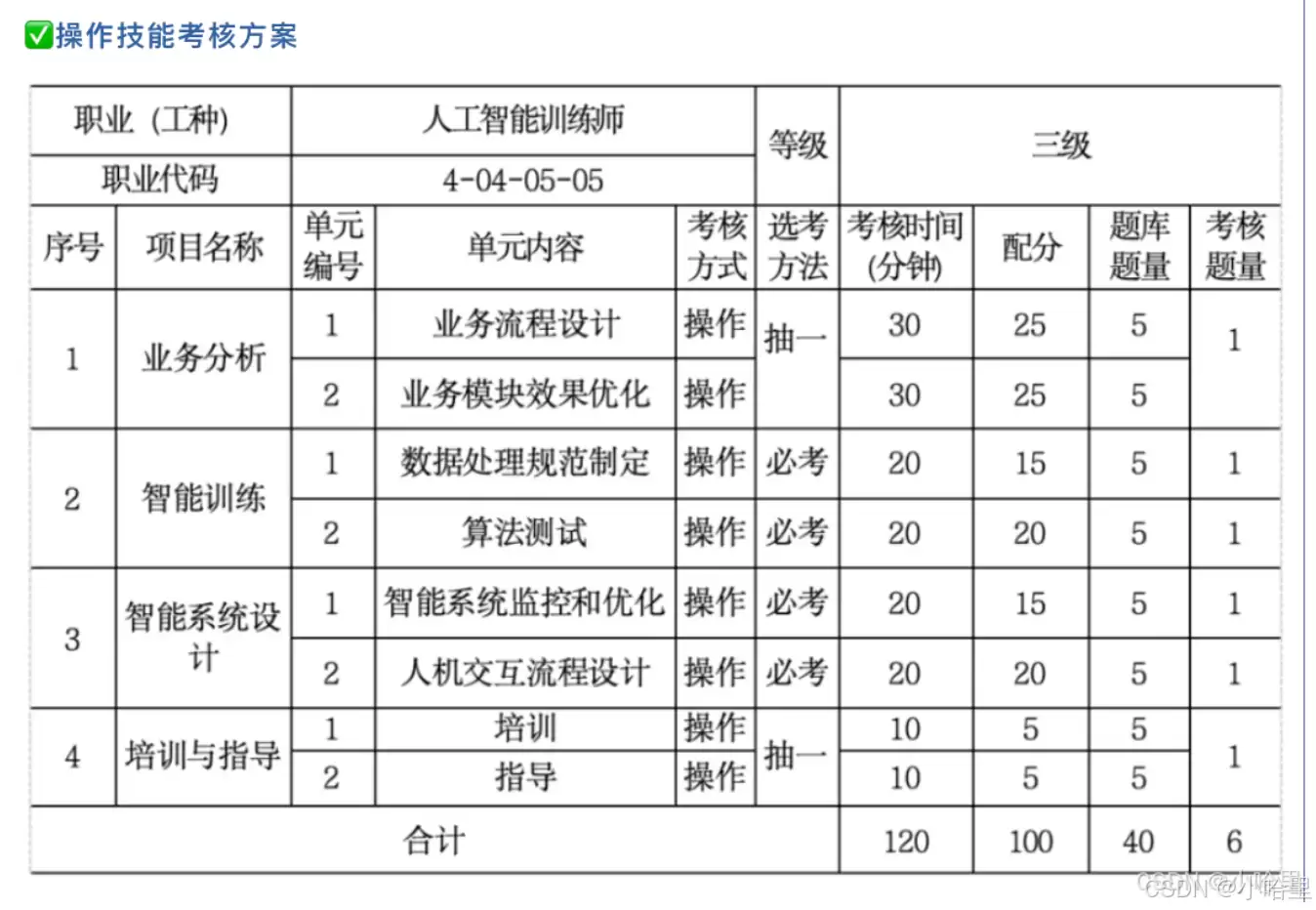
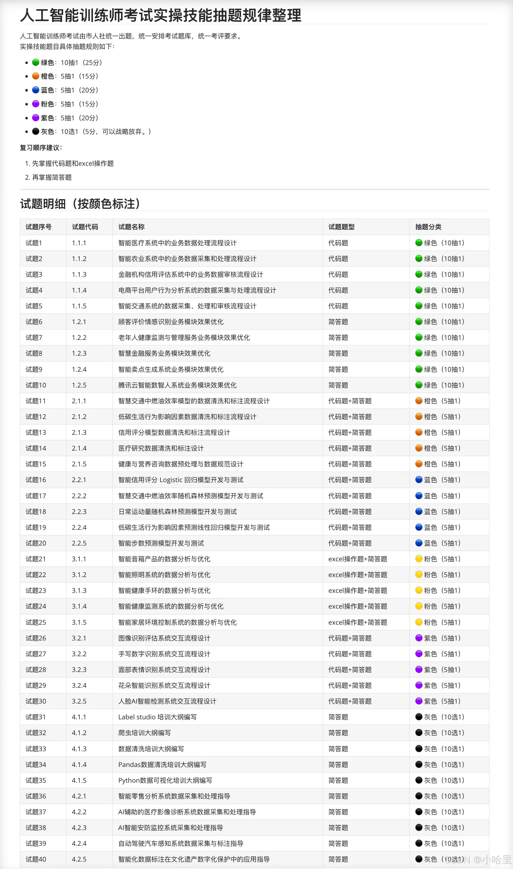
3、其实操作技能和理论知识都是原题题库抽的,然后原题是官方发出来了的,就是没有答案,自己做一遍背一下就好了。
视频课推荐B站的 北魏乔木
import cv2import matplotlib.pyplot as pltimport numpy as npimport onnxruntime as ortimport pandas as pdimport scipy.specialfrom imblearn.over_sampling import SMOTEfrom PIL import Imagefrom sklearn.linear_model import LogisticRegressionfrom xgboost import XGBRegressor# =========================# 1. 数据读取与基础清洗# =========================# 读取医疗数据,注意中文编码可能使用 gbk。data = pd.read_csv("medical_data.csv", encoding="gbk")# 重命名列名,便于后续分析。data.rename(columns={"病人ID":"患者ID"}, inplace=True)# 查看原始行数,方便对比清洗前后数据量变化。initial_row_count = data.shape[0]# 统计重复值数量。duplicate_values = data.duplicated().sum()# 删除重复数据。data = data.drop_duplicates()# 性别字段统一编码。data["Gender"]= data["Gender"].replace({"M":"Male","F":"Female"})data["Gender"]= data["Gender"].fillna("Male")# 吸烟字段按映射字典统一取值。data["Smoking"]= data["Smoking"].replace(smoking_mapping)# 将分类变量转换为哑变量。data_cleaned = pd.get_dummies(data, drop_first=True)# =========================# 2. 特征处理与数值转换# =========================# 将字符串型数值转换为真正的数值,无法转换的记为 NaN。df["horsepower"]= pd.to_numeric(df["horsepower"], errors="coerce")# 将分类变量转成数值变量,便于模型训练。X = pd.get_dummies(X)# 将年龄段文本提取为整数,例如 "25 years" 提取为 25。y = df["Your age"].apply(lambda x:int(x.split(" ")[0]))# 数值特征标准化。data[numerical_features]= scaler.fit_transform(data[numerical_features])# 也可以单独查看标准化结果。scaled_values = scaler.fit_transform(data[numerical_features])# 合并处理后的特征和标签。cleaned_data = pd.concat([X, y], axis=1)# 计算四分位数,常用于异常值检测。Q1 = data[numeric_cols].quantile(0.25)# =========================# 3. 条件筛选与分组统计# =========================# 从传感器类型中筛选温度和湿度数据。sensor_subset = data[data["SensorType"].isin(["Temperature","Humidity"])]# 根据住院天数生成风险等级标签。data["RiskLevel"]= np.where(data["DaysInHospital"]>60,"高风险","低风险")# 对每组 Value 同时计算数量和均值。group_stats = data.groupby("Value").agg(["count","mean"])# =========================# 4. 类别不平衡处理与传统模型# =========================# 使用 SMOTE 对训练集进行过采样,缓解类别不平衡问题。smote = SMOTE(random_state=42)X_train_resampled, y_train_resampled = smote.fit_resample(X_train, y_train)# 逻辑回归模型,适合做二分类任务。model = LogisticRegression(max_iter=1000)model.fit(X_train_resampled, y_train_resampled)# 计算预测准确率。accuracy =(y_test == y_pred).mean()# =========================# 5. XGBoost 回归模型# =========================# 基础版 XGBoost 回归器。xgb_model = XGBRegressor(n_estimators=100, random_state=42)xgb_model.fit(X_train, y_train)# 查看训练集得分。train_score = xgb_model.score(X_train, y_train)# 进阶版参数设置,通过增加树数量、降低学习率来提升拟合效果。xgb_model = XGBRegressor(n_estimators=1000,learning_rate=0.05,max_depth=5,subsample=0.8,colsample_bytree=0.8,random_state=42,)# 保存预测结果,便于对比实际值与预测值。results = pd.DataFrame({"实际值": y_test,"预测值": y_pred})# =========================# 6. 图像读取与 ONNX 推理# =========================# 读取原始图片。orig_image = cv2.imread(img_path)# 使用 PIL 打开测试图片并转换为 RGB。image = Image.open("img_test.jpg").convert("RGB")# 转为 numpy 数组,并指定 float32 类型。image_array = np.array(image, dtype=np.float32)# 如果变量名已经是 numpy 数组,也可以直接转换类型。image_array = image_array.astype(np.float32)processed_image = processed_image.astype(np.float32)# 增加 batch 维度,满足模型输入要求。image_array = np.expand_dims(image_array, axis=0)# 创建 ONNX 推理会话。session = ort.InferenceSession("resnet.onnx")# 获取模型输入输出名称。input_name = session.get_inputs()[0].nameoutput_name = session.get_outputs()[0].name# 模型推理。output = session.run([output_name],{input_name: processed_image})[0]# 对输出结果做 softmax,转换为概率。probabilities = scipy.special.softmax(output, axis=-1)# 获取概率最高的前 5 个类别下标和对应概率。top5_idx = np.argsort(probabilities[0])[-5:][::-1]top5_prob = probabilities[0][top5_idx]# 读取标签文件。withopen("labels.txt","r", encoding="utf-8")as f:labels =[line.strip()for line in f.readlines()]# np.argsort 默认是从小到大排序并返回下标。# =========================# 7. 可视化分析# =========================plt.figure(figsize=(10,6))# 散点图:观察年龄与疾病严重程度关系。plt.scatter(data["年龄"], data["疾病严重程度"])# 堆叠柱状图:展示不同治疗结果分布。treatment_outcome_distribution.plot(kind="bar", stacked=True)# 饼图:展示运动频率占比。exercise_frequency_counts.plot.pie(autopct="%1.1f%%",startangle=90,colors=plt.cm.Paired.colors,)# =========================# 8. 零散知识点备注# =========================# n_estimators=100# 表示模型中树的数量为 100,常见于随机森林或 XGBoost。# duplicated()# 用于判断每一行是否重复,返回布尔序列。# data.duplicated().sum()# 用于统计重复行的总数量。# pd.to_numeric(..., errors="coerce")# 无法转换的值会被强制设为 NaN。# pd.get_dummies(...)# 用于将分类变量转换为数值型哑变量。# %% [markdown]# # 1.1.1# # %% [markdown]# ## 1.1.1 素材# # `1.1.1/1.1.1.ipynb`# # %%import pandas as pdimport numpy as np# 读取数据集 1分data = _____________# %%# 1. 统计住院天数超过7天的患者数量及其占比# 创建新列'RiskLevel',根据住院天数判断风险等级 3分_____________ = _____________(_____________,'高风险患者','低风险患者')# 统计不同风险等级的患者数量 2分risk_counts = data_____________._____________# 计算高风险患者占比 1分high_risk_ratio = risk_counts['高风险患者']/ _____________# 计算低风险患者占比 1分low_risk_ratio = risk_counts['低风险患者']/ _____________# 输出结果print("高风险患者数量:", risk_counts['高风险患者'])print("低风险患者数量:", risk_counts['低风险患者'])print("高风险患者占比:", high_risk_ratio)print("低风险患者占比:", low_risk_ratio)# %%# 2. 统计不同BMI区间中高风险患者的比例和统计不同BMI区间中的患者数# 定义BMI区间和标签bmi_bins =[0,18.5,24,28, np.inf]bmi_labels =['偏瘦','正常','超重','肥胖']# 根据BMI值划分指定区间 4分data['BMIRange']= _____________(_____________, _____________, _____________, right=False)# 使用左闭右开区间# 计算每个BMI区间中高风险患者的比例 2分bmi_risk_rate = _____________(_____________)['RiskLevel'].apply(lambda x:(x =='高风险患者').mean())# 统计每个BMI区间的患者数量 1分bmi_patient_count = data_____________# 输出结果print("BMI区间中高风险患者的比例和患者数:")print(bmi_risk_rate)print(bmi_patient_count)# %%# 3. 统计不同年龄区间中高风险患者的比例和统计不同年龄区间中的患者数# 定义年龄区间和标签age_bins =[0,26,36,46,56,66, np.inf]age_labels =['≤25岁','26-35岁','36-45岁','46-55岁','56-65岁','>65岁']# 根据年龄值划分指定区间 4分data['AgeRange']= _____________(_____________, _____________, _____________, right=False)# 使用左闭右开区间# 计算每个年龄区间中高风险患者的比例 2分age_risk_rate = _____________(_____________)['RiskLevel'].apply(lambda x:(x =='高风险患者').mean())# 统计每个年龄区间的患者数量 1分age_patient_count = data_____________# 输出结果print("年龄区间中高风险患者的比例和患者数:")print(age_risk_rate)print(age_patient_count)# %% [markdown]# ## 1.1.1 答案# # `1.1.1答案/1.1.1.ipynb`# # %%import pandas as pdimport numpy as np# 读取数据集 1分data = pd.read_csv('patient_data.csv')# %%# 1. 统计住院天数超过7天的患者数量及其占比# 创建新列'RiskLevel',根据住院天数判断风险等级 3分data['RiskLevel']=np.where(data['DaysInHospital']>7,'高风险患者','低风险患者')# 统计不同风险等级的患者数量 2分risk_counts = data['RiskLevel'].value_counts()# 计算高风险患者占比 1分high_risk_ratio = risk_counts['高风险患者']/len(data)# 计算低风险患者占比 1分low_risk_ratio = risk_counts['低风险患者']/len(data)# 输出结果print("高风险患者数量:", risk_counts['高风险患者'])print("低风险患者数量:", risk_counts['低风险患者'])print("高风险患者占比:", high_risk_ratio)print("低风险患者占比:", low_risk_ratio)# %%# 2. 统计不同BMI区间中高风险患者的比例和统计不同BMI区间中的患者数# 定义BMI区间和标签bmi_bins =[0,18.5,24,28, np.inf]bmi_labels =['偏瘦','正常','超重','肥胖']# 根据BMI值划分指定区间 4分data['BMIRange']= pd.cut(data['BMI'], bins=bmi_bins, labels=bmi_labels, right=False)# 使用左闭右开区间# 计算每个BMI区间中高风险患者的比例 2分bmi_risk_rate =data.groupby('BMIRange')['RiskLevel'].apply(lambda x:(x =='高风险患者').mean())# 统计每个BMI区间的患者数量 1分bmi_patient_count = data['BMIRange'].value_counts()# 输出结果print("BMI区间中高风险患者的比例和患者数:")print(bmi_risk_rate)print(bmi_patient_count)# %%# 3. 统计不同年龄区间中高风险患者的比例和统计不同年龄区间中的患者数# 定义年龄区间和标签age_bins =[0,26,36,46,56,66, np.inf]age_labels =['≤25岁','26-35岁','36-45岁','46-55岁','56-65岁','>65岁']# 根据年龄值划分指定区间 4分data['AgeRange']= pd.cut(data['Age'], bins=age_bins, labels=age_labels,right=False)# 使用左闭右开区间)# 计算每个年龄区间中高风险患者的比例 2分age_risk_rate = data.groupby('AgeRange')['RiskLevel'].apply(lambda x:(x =='高风险患者').mean())# 统计每个年龄区间的患者数量 1分age_patient_count = data['AgeRange'].value_counts()# 输出结果print("年龄区间中高风险患者的比例和患者数:")print(age_risk_rate)print(age_patient_count)# %%# %% [markdown]# ---# # %% [markdown]# # 1.1.2# # %% [markdown]# ## 1.1.2 素材# # `1.1.2/1.1.2.ipynb`# # %%import pandas as pdimport numpy as npimport matplotlib.pyplot as plt# 读取数据集 2分data = _____________# %%# 1. 传感器数据统计# 对传感器类型进行分组,并计算每个组的数据数量和平均值 3分sensor_stats = _____________(_____________)['Value']._____________# 输出结果print("传感器数据数量和平均值:")print(sensor_stats)# %%# 2. 按位置统计温度和湿度数据# 筛选出温度和湿度数据,然后按位置和传感器类型分组,计算每个组的平均值 2分location_stats = data[data['SensorType']._____________._____________['Value'].mean().unstack()# 输出结果print("每个位置的温度和湿度数据平均值:")print(location_stats)# %%# 3. 数据清洗和异常值处理# 标记异常值 3分data['is_abnormal']= _____________(((_____________)&((data['Value']<-10)|(data['Value']>50)))|((_____________)&((data['Value']<0)|(data['Value']>100))),True,False)# 输出异常值数量 2分print("异常值数量:", data['is_abnormal']._____________)# 填补缺失值# 使用前向填充和后向填充的方法填补缺失值 4分data['Value']._____________(_____________, inplace=True)data['Value']._____________(_____________, inplace=True)# 保存清洗后的数据# 删除用于标记异常值的列,并将清洗后的数据保存到新的CSV文件中 4分cleaned_data = _____________(_____________=['is_abnormal'])_____________('cleaned_sensor_data.csv', _____________)print("数据清洗完成,已保存为 'cleaned_sensor_data.csv'")# %% [markdown]# ## 1.1.2 答案# # `1.1.2答案/1.1.2.ipynb`# # %%import pandas as pdimport numpy as npimport matplotlib.pyplot as plt# 读取数据集data = pd.read_csv('sensor_data.csv')# %%# 1. 传感器数据统计# 对传感器类型进行分组,并计算每个组的数据数量和平均值sensor_stats = data.groupby('SensorType')['Value'].agg(['count','mean'])# 输出结果print("传感器数据数量和平均值:")print(sensor_stats)# %%# 2. 按位置统计温度和湿度数据# 筛选出温度和湿度数据,然后按位置和传感器类型分组,计算每个组的平均值location_stats = data[data['SensorType'].isin(['Temperature','Humidity'])].groupby(['Location','SensorType'])['Value'].mean().unstack()# 输出结果print("每个位置的温度和湿度数据平均值:")print(location_stats)# %%# 3. 数据清洗和异常值处理# 标记异常值data['is_abnormal']= np.where(((data['SensorType']=='Temperature')&((data['Value']<-10)|(data['Value']>50)))|((data['SensorType']=='Humidity')&((data['Value']<0)|(data['Value']>100))),True,False)# 输出异常值数量print("异常值数量:", data['is_abnormal'].sum())# 填补缺失值# 使用前向填充和后向填充的方法填补缺失值data['Value'].fillna(method='ffill', inplace=True)data['Value'].fillna(method='bfill', inplace=True)# 保存清洗后的数据# 删除用于标记异常值的列,并将清洗后的数据保存到新的CSV文件中cleaned_data = data.drop(columns=['is_abnormal'])cleaned_data.to_csv('cleaned_sensor_data.csv', index=False)print("数据清洗完成,已保存为 'cleaned_sensor_data.csv'")# %%# %% [markdown]# ---# # %% [markdown]# # 1.1.3# # %% [markdown]# ## 1.1.3 素材# # `1.1.3/1.1.3.ipynb`# # %%import pandas as pdimport numpy as npimport matplotlib.pyplot as plt# 读取数据集data = pd.read_csv('credit_data.csv')# %%# 1. 数据完整性审核missing_values = data._________ #数据缺失值统计 2分duplicate_values = data._________ #数据重复值统计 2分# 输出结果print("缺失值统计:")print(missing_values)print("重复值统计:")print(duplicate_values)# %%# 2. 数据合理性审核data['is_age_valid']= _________._________(18,70)#Age数据的合理性审核 2分data['is_income_valid']= _________ > _________ #Income数据的合理性审核 2分data['is_loan_amount_valid']= _________ <(_________ *5)#LoanAmount数据的合理性审核 2分data['is_credit_score_valid']= _________._________(300,850)#CreditScore数据的合理性审核 2分# 合理性检查结果validity_checks = data[['is_age_valid','is_income_valid','is_loan_amount_valid','is_credit_score_valid']].all(axis=1)data['is_valid']= validity_checks# 输出结果print("数据合理性检查:")print(data[['is_age_valid','is_income_valid','is_loan_amount_valid','is_credit_score_valid','is_valid']].describe())# %%# 3. 数据清洗和异常值处理# 标记不合理数据invalid_rows = data[~data['is_valid']]# 删除不合理数据行cleaned_data = data[data['is_valid']]# 删除标记列cleaned_data = cleaned_data.drop(columns=['is_age_valid','is_income_valid','is_loan_amount_valid','is_credit_score_valid','is_valid'])# 保存清洗后的数据_________._________(_________, index=False)print("数据清洗完成,已保存为 'cleaned_credit_data.csv'")# %% [markdown]# ## 1.1.3 答案# # `1.1.3答案/1.1.3.ipynb`# # %%import pandas as pdimport numpy as npimport matplotlib.pyplot as plt# 读取数据集data = pd.read_csv('credit_data.csv')# %%# 1. 数据完整性审核missing_values = data.isna().sum()#数据缺失值统计 2分duplicate_values = data.duplicated().sum()#数据重复值统计 2分# 输出结果print("缺失值统计:")print(missing_values)print("重复值统计:")print(duplicate_values)# %%# 2. 数据合理性审核data['is_age_valid']= data['Age'].between(18,70)#Age数据的合理性审核 2分data['is_income_valid']= data['Income']>2000#Income数据的合理性审核 2分data['is_loan_amount_valid']= data['LoanAmount']<(data['Income']*5)#LoanAmount数据的合理性审核 2分data['is_credit_score_valid']= data['CreditScore'].between(300,850)#CreditScore数据的合理性审核 2分# 合理性检查结果validity_checks = data[['is_age_valid','is_income_valid','is_loan_amount_valid','is_credit_score_valid']].all(axis=1)data['is_valid']= validity_checks# 输出结果print("数据合理性检查:")print(data[['is_age_valid','is_income_valid','is_loan_amount_valid','is_credit_score_valid','is_valid']].describe())# %%# 3. 数据清洗和异常值处理# 标记不合理数据invalid_rows = data[~data['is_valid']]# 删除不合理数据行cleaned_data = data[data['is_valid']]# 删除标记列cleaned_data = cleaned_data.drop(columns=['is_age_valid','is_income_valid','is_loan_amount_valid','is_credit_score_valid','is_valid'])# 保存清洗后的数据cleaned_data.to_csv('cleaned_credit_data.csv', index=False)print("数据清洗完成,已保存为 'cleaned_credit_data.csv'")# %%# %% [markdown]# ---# # %% [markdown]# # 1.1.4# # %% [markdown]# ## 1.1.4 素材# # `1.1.4/1.1.4.ipynb`# # %%import pandasimport numpy as npimport matplotlib.pyplot as plt# 1. 数据采集# 从本地文件中读取数据2分data =_______________________________print("数据采集完成,已加载到DataFrame中")# 打印数据的前5条记录2分print(________________________________)# %%# 2. 数据清洗与预处理# 处理缺失值(删除)2分data = ________________________________# 数据类型转换data________________ = ________________(int)# Age数据类型转换为int 2分data________________ = ________________(float)# PurchaseAmount数据类型转换为float2分data________________ = ________________(int)# ReviewScore数据类型转换为int 2分# 处理异常值2分data = data[(________________.________________(18,70))&(data['PurchaseAmount']>0)&(________________.________________(1,5))]# 数据标准化data['PurchaseAmount']=(data['PurchaseAmount']- ________________)/ ________________# PurchaseAmount数据标准化 2分data['ReviewScore']=(data['ReviewScore']- ________________)/ ________________# ReviewScore数据标准化 2分# 保存清洗后的数据1分________________('cleaned_user_behavior_data.csv', index=False)print("数据清洗完成,已保存为 'cleaned_user_behavior_data.csv'")# %%# 3. 数据统计# 统计每个购买类别的用户数 2分purchase_category_counts = ________________.________________print("每个购买类别的用户数:n", purchase_category_counts)# 统计不同性别的平均购买金额 2分gender_purchase_amount_mean = ________________(________________)['PurchaseAmount'].mean()print("不同性别的平均购买金额:n", gender_purchase_amount_mean)# 统计不同年龄段的用户数 2分bins =[18,26,36,46,56,66, np.inf]labels =['18-25','26-35','36-45','46-55','56-65','65+']data['AgeGroup']= pandas.________________(________________, right=False)age_group_counts = data['AgeGroup'].value_counts().sort_index()print("不同年龄段的用户数:n", age_group_counts)# %% [markdown]# ## 1.1.4 答案# # `1.1.4 答案/1.1.4.ipynb`# # %%import pandasimport numpy as npimport matplotlib.pyplot as plt# 1. 数据采集# 从本地文件中读取数据2分data =pandas.read_csv('user_behavior_data.csv')print("数据采集完成,已加载到DataFrame中")# 打印数据的前5条记录2分print(data.head(5))# %%# 2. 数据清洗与预处理# 处理缺失值2分data = data.dropna()# 数据类型转换data['Age']= data['Age'].astype(int)# Age数据类型转换 2分data['PurchaseAmount']= data['PurchaseAmount'].astype(float)# PurchaseAmount数据类型转换2分data['ReviewScore']= data['ReviewScore'].astype(int)# ReviewScore数据类型转换 2分# 处理异常值2分data = data[(data['Age'].between(18,70))&(data['PurchaseAmount']>0)&(data['ReviewScore'].between(1,5))]# 数据标准化data['PurchaseAmount']=(data['PurchaseAmount']- data['PurchaseAmount'].mean())/ data['PurchaseAmount'].std()# PurchaseAmount数据标准化 2分data['ReviewScore']=(data['ReviewScore']- data['ReviewScore'].mean())/ data['ReviewScore'].std()# ReviewScore数据标准化 2分# 保存清洗后的数据1分data.to_csv('cleaned_user_behavior_data.csv', index=False)print("数据清洗完成,已保存为 'cleaned_user_behavior_data.csv'")# %%# 3. 数据统计# 统计每个购买类别的用户数purchase_category_counts = data['PurchaseCategory'].value_counts()print("每个购买类别的用户数:n", purchase_category_counts)# 统计不同性别的平均购买金额gender_purchase_amount_mean = data.groupby('Gender')['PurchaseAmount'].mean()print("不同性别的平均购买金额:n", gender_purchase_amount_mean)# 统计不同年龄段的用户数bins =[18,26,36,46,56,66, np.inf]labels =['18-25','26-35','36-45','46-55','56-65','65+']data['AgeGroup']= pandas.cut(data['Age'], bins=bins, labels=labels, right=False)age_group_counts = data['AgeGroup'].value_counts().sort_index()print("不同年龄段的用户数:n", age_group_counts)# %%# %%# %% [markdown]# ---# # %% [markdown]# # 1.1.5# # %% [markdown]# ## 1.1.5 素材# # `1.1.5/1.1.5.ipynb`# # %%import pandas as pdimport numpy as npimport matplotlib.pyplot as plt# 1. 数据采集# 从本地文件中读取数据2分data = _____________print("数据采集完成,已加载到DataFrame中")# 打印数据的前5条记录 2分print(_____________)# %%# 2. 数据清洗与预处理# 处理缺失值(删除)2分data = _____________# 数据类型转换data_____________ = _____________(int)#Age数据类型转换为int 1分data_____________ = _____________(float)#Speed数据类型转换为float 1分data_____________ = _____________(float)#TravelDistance数据类型转换为float 1分data_____________ = _____________(float)#TravelTime数据类型转换为float 1分# 处理异常值2分data = data[(_____________(18,70))&(_____________(0,200))&(_____________(1,1000))&(_____________(1,1440))]# 保存清洗后的数据1分_____________('cleaned_vehicle_traffic_data.csv', index=False)print("数据清洗完成,已保存为 'cleaned_vehicle_traffic_data.csv'")# %%# 3. 数据合理性审核# 审核字段合理性 1分unreasonable_data = data[~((_____________(18,70))&(_____________(0,200))&(_____________(1,1000))&(_____________(1,1440)))]print("不合理的数据:n", unreasonable_data)# 4. 数据统计# 统计每种交通事件的发生次数2分traffic_event_counts = _____________print("每种交通事件的发生次数:n", traffic_event_counts)# 统计不同性别的平均车速、行驶距离和行驶时间2分gender_stats = data._____________._____________print("不同性别的平均车速、行驶距离和行驶时间:n", gender_stats)# 统计不同年龄段的驾驶员数5分age_bins =[18,26,36,46,56,66, np.inf]age_labels =['18-25','26-35','36-45','46-55','56-65','65+']data['AgeGroup']= _____________(_____________,_____________,_____________, right=False)age_group_counts = _____________print("不同年龄段的驾驶员数:n", age_group_counts)# %% [markdown]# ## 1.1.5 答案# # `1.1.5 答案/1.1.5.ipynb`# # %%import pandas as pdimport numpy as npimport matplotlib.pyplot as plt# 1. 数据采集# 从本地文件中读取数据2分data = pd.read_csv('vehicle_traffic_data.csv')print("数据采集完成,已加载到DataFrame中")# 打印数据的前5条记录print(data.head(5))# %%# 2. 数据清洗与预处理# 处理缺失值2分data = data.dropna()# 数据类型转换data['Age']= data['Age'].astype(int)#Age数据类型转换 1分data['Speed']= data['Speed'].astype(float)#Speed数据类型转换 1分data['TravelDistance']= data['TravelDistance'].astype(float)#TravelDistance数据类型转换 1分data['TravelTime']= data['TravelTime'].astype(float)#TravelTime数据类型转换 1分# 处理异常值2分data = data[(data['Age'].between(18,70))&(data['Speed'].between(0,200))&(data['TravelDistance'].between(1,1000))&(data['TravelTime'].between(1,1440))]# 保存清洗后的数据1分data.to_csv('cleaned_vehicle_traffic_data.csv', index=False)print("数据清洗完成,已保存为 'cleaned_vehicle_traffic_data.csv'")# %%# 3. 数据合理性审核# 审核字段合理性 1分unreasonable_data = data[~((data['Age'].between(18,70))&(data['Speed'].between(0,200))&(data['TravelDistance'].between(1,1000))&(data['TravelTime'].between(1,1440)))]print("不合理的数据:n", unreasonable_data)# 4. 数据统计# 统计每种交通事件的发生次数2分traffic_event_counts = data['TrafficEvent'].value_counts()print("每种交通事件的发生次数:n", traffic_event_counts)# 统计不同性别的平均车速、行驶距离和行驶时间2分gender_stats = data.groupby('Gender').agg({'Speed':'mean','TravelDistance':'mean','TravelTime':'mean'})print("不同性别的平均车速、行驶距离和行驶时间:n", gender_stats)# 统计不同年龄段的驾驶员数2分age_bins =[18,26,36,46,56,66, np.inf]age_labels =['18-25','26-35','36-45','46-55','56-65','65+']data['AgeGroup']= pd.cut(data['Age'], bins=age_bins, labels=age_labels, right=False)age_group_counts = data['AgeGroup'].value_counts().sort_index()print("不同年龄段的驾驶员数:n", age_group_counts)# %%# %% [markdown]# ---# # %% [markdown]# # 1.1.6# # %% [markdown]# ## 1.1.6 素材# # `1.1.6-未公开流出版/1.1.6代码-流出版.ipynb`# # %% [markdown]# # 1.1.6 电商用户行为数据分析# # 你是一家电商平台的数据分析师,现有一份用户行为数据文件 ecommerce_user_data.csv,包含以下字段:# # | 字段名 | 含义 | 示例 |# |---|---|---|# | UserID | 用户唯一标识 | 1001 |# | UserName | 用户名 | User_1 |# | Age | 年龄(可能存在缺失或异常值) | 23 |# | Gender | 性别(Male/Female) | Male |# | PurchaseAmount | 购买金额(单位:元,可能为负数或异常高值) | 899.5 |# | ProductCategory | 购买商品类别(Electronics, Clothing, Books, Home, Sports) | Electronics |# | Rating | 用户评分(1-5分,可能超出范围) | 4 |# | LoginFrequency | 登录频率(Daily, Weekly, Monthly) | Weekly |# | LastPurchaseDate | 最近一次购买日期 | 2023-07-15 |# # 请完成以下三个任务:# # **1. 数据采集与初步查看**# - 使用 pandas 读取 ecommerce_user_data.csv 文件# - 打印数据的前5行,确认数据已正确加载# # **2. 数据清洗与预处理**# - 处理缺失值:删除含有缺失值的行# - 数据类型转换:# - Age 转为整型# - PurchaseAmount 转为浮点型# - Rating 转为整型# - 处理异常值:# - 年龄应在 18~70 岁之间# - 购买金额应大于 0# - 评分应在 1~5 之间# - 新增字段:# - 创建 AgeGroup 字段,将用户划分为年龄段:# - 18-25: 18~25岁# - 26-35: 26~35岁# - 36-45: 36~45岁# - 46-55: 46~55岁# - 56+: 56岁及以上# - 将清洗后的数据保存为 cleaned_ecommerce_data.csv# # **3. 数据统计分析**# - 统计每个商品类别的购买人数# - 计算不同性别的平均购买金额# - 统计各年龄段的用户数量,并按年龄段排序输出# %%# 1. 数据采集data = _____________print("数据采集完成,已加载到DataFrame中")#显示前五行数据print(_____________)# 2. 数据清洗与预处理# 处理缺失值data = _____________# 数据类型转换_____________ = _____________ #Age数据类型转换为int_____________ = _____________ #PurchaseAmount数据类型转换为float_____________ = _____________ #Rating数据类型转换为int# 处理异常值data = data[ data['Age']_____________(18,70)&(data['PurchaseAmount']>0)& data['Rating']_____________(1,5)]# 新增 AgeGroup 字段bins =[18,25,35,45,55,70]labels =['18-25','26-35','36-45','46-55','56+']data['AgeGroup']= _____________ (_____________, _____________, _____________, right=True)# 保存清洗后数据_____________('cleaned_ecommerce_data.csv', _____________)print("数据清洗完成,已保存为 'cleaned_ecommerce_data.csv'")# 3. 数据统计分析# 每个商品类别的购买人数category_count = _____________print("n每个商品类别的购买人数:n", category_count)# 不同性别的平均购买金额avg_purchase_by_gender = _____________print("n不同性别的平均购买金额:n", avg_purchase_by_gender)# 各年龄段用户数量age_group_count = _____________.sort_index()print("n各年龄段的用户数量:n", age_group_count)# %%# %% [markdown]# ## 1.1.6 答案# # `1.1.6流出版-答案/1.1.6流出版-答案.ipynb`# # %%import pandas as pdimport numpy as np# 1. 数据采集data = pd.read_csv('ecommerce_user_data.csv')print("数据采集完成,已加载到DataFrame中")print(data.head())# 2. 数据清洗与预处理# 处理缺失值data = data.dropna()# 数据类型转换data['Age']= data['Age'].astype(int)data['PurchaseAmount']= data['PurchaseAmount'].astype(float)data['Rating']= data['Rating'].astype(int)# 处理异常值data = data[data['Age'].between(18,70)&(data['PurchaseAmount']>0)&data['Rating'].between(1,5)]# 新增 AgeGroup 字段bins =[18,25,35,45,55,70]labels =['18-25','26-35','36-45','46-55','56+']data['AgeGroup']= pd.cut(data['Age'], bins=bins, labels=labels, right=True)# 保存清洗后数据data.to_csv('cleaned_ecommerce_data.csv', index=False)print("数据清洗完成,已保存为 'cleaned_ecommerce_data.csv'")# 3. 数据统计分析# 每个商品类别的购买人数category_count = data['ProductCategory'].value_counts()print("n每个商品类别的购买人数:n", category_count)# 不同性别的平均购买金额avg_purchase_by_gender = data.groupby('Gender')['PurchaseAmount'].mean()print("n不同性别的平均购买金额:n", avg_purchase_by_gender)# 各年龄段用户数量age_group_count = data['AgeGroup'].value_counts().sort_index()print("n各年龄段的用户数量:n", age_group_count)# %%# %% [markdown]# ---# # %% [markdown]# # 2.1.1# # %% [markdown]# ## 2.1.1 素材# # `2.1.1/2.1.1.ipynb`# # %%import pandas as pd# 加载数据集并显示数据集的前五行 1分data = __________print("数据集的前五行:")print(__________)# 显示每一列的数据类型print(data.dtypes)# 检查缺失值并删除缺失值所在的行2分print("n检查缺失值:")print(__________.__________.__________)data = __________# 将 'horsepower' 列转换为数值类型,并(删除)处理转换中的异常值 1分data['horsepower']= __________(data['horsepower'], errors='coerce')data = __________# 显示每一列的数据类型print(data.horsepower.dtypes)# 检查清洗后的缺失值print("n检查清洗后的缺失值:")print(data.isnull().sum())from sklearn.preprocessing import StandardScaler# 对数值型数据进行标准化处理 1分numerical_features =['displacement','horsepower','weight','acceleration']scaler = StandardScaler()data[numerical_features]= __________from sklearn.model_selection import train_test_split# 选择特征、自变量和目标变量 2分selected_features = __________X = __________y = __________# 划分数据集为训练集和测试集(训练集占8成) 1分X_train, X_test, y_train, y_test = __________(__________, random_state=42)# 将特征和目标变量合并到一个数据框中cleaned_data = X.copy()cleaned_data['mpg']= y# 保存清洗和处理后的数据(不存储额外的索引号) 1分__________('2.1.1_cleaned_data.csv', __________)# 打印消息指示文件已保存print("n清洗后的数据已保存到 2.1.1_cleaned_data.csv")# %%# %% [markdown]# ## 2.1.1 答案# # `2.1.1答案/2.1.1.ipynb`# # %%import pandas as pd# 加载数据集并显示数据集的前五行 1分data = pd.read_csv('auto-mpg.csv')print("数据集的前五行:")print(data.head())# 显示每一列的数据类型print(data.dtypes)# 检查缺失值并删除缺失值所在的行2分print("n检查缺失值:")print(data.isnull().sum())data = data.dropna()# 将 'horsepower' 列转换为数值类型,并处理转换中的异常值 1分data['horsepower']= pd.to_numeric(data['horsepower'], errors='coerce')data = data.dropna(subset=['horsepower'])# 显示每一列的数据类型print(data.horsepower.dtypes)# 检查清洗后的缺失值print("n检查清洗后的缺失值:")print(data.isnull().sum())from sklearn.preprocessing import StandardScaler# 对数值型数据进行标准化处理 1分numerical_features =['displacement','horsepower','weight','acceleration']scaler = StandardScaler()data[numerical_features]= scaler.fit_transform(data[numerical_features])from sklearn.model_selection import train_test_split# 选择特征和目标变量 2分selected_features =['cylinders','displacement','horsepower','weight','acceleration','model year','origin']X = data[selected_features]y = data['mpg']# 划分数据集为训练集和测试集 1分X_train, X_test, y_train, y_test = train_test_split(X, y, test_size=0.2, random_state=42)# 将特征和目标变量合并到一个数据框中cleaned_data = X.copy()cleaned_data['mpg']= y# 保存清洗和处理后的数据cleaned_data.to_csv('2.1.1_cleaned_data.csv', index=False)# 打印消息指示文件已保存print("n清洗后的数据已保存到 2.1.1_cleaned_data.csv")# %%# %% [markdown]# ---# # %% [markdown]# # 2.1.2# # %% [markdown]# ## 2.1.2 素材# # `2.1.2/2.1.2.ipynb`# # %%import pandas as pd#读取一个Excel文件,并将读取到的数据存储在变量data中data = __________#打印出数据集的前5行print(data.head())#处理数据集中的缺失值initial_row_count = __________ #处理前的数据行数data = __________#删除缺失值所在行final_row_count = __________ #处理后的数据行数print(f'处理后数据行数: {final_row_count}, 删除的行数: {initial_row_count - final_row_count}')#删除重复行data = __________from sklearn.preprocessing import StandardScalernumerical_features =['4.您的月生活费○≦1,000元 ○1,001-2,000元 ○2,001-3,000元 ○≧3,001元']scaler = StandardScaler()data[numerical_features]= __________#选择特征selected_features =[__________]X = __________# 创建目标变量y = __________from sklearn.model_selection import train_test_split# 数据划分(测试集取20%)X_train, X_test, y_train, y_test = __________(__________, random_state=42)# 合并处理后得数据,并将其保存(保存中不用额外创建索引)cleaned_data = __________(__________, axis=1)__________('2.1.2_cleaned_data.csv', __________)# %%# %% [markdown]# ## 2.1.2 答案# # `2.1.2答案/2.1.2.ipynb`# # %%import pandas as pdfrom sklearn.preprocessing import StandardScalerfrom sklearn.model_selection import train_test_split#读取一个Excel文件,并将读取到的数据存储在变量data中data = pd.read_excel('大学生低碳生活行为的影响因素数据集.xlsx')#打印出数据集的前5行print(data.head())#处理数据集中的缺失值initial_row_count = data.shape[0]data = data.dropna()final_row_count = data.shape[0]print(f'处理后数据行数: {final_row_count}, 删除的行数: {initial_row_count - final_row_count}')#删除重复行data =data.drop_duplicates()from sklearn.preprocessing import StandardScalernumerical_features =['4.您的月生活费○≦1,000元 ○1,001-2,000元 ○2,001-3,000元 ○≧3,001元']scaler = StandardScaler()data[numerical_features]= scaler.fit_transform(data[numerical_features])selected_features =['1.您的性别○男性 ○女性','2.您的年级○大一 ○大二 ○大三 ○大四','3.您的生源地○农村 ○城镇(乡镇) ○地县级城市○省会城市及直辖市','4.您的月生活费○≦1,000元 ○1,001-2,000元 ○2,001-3,000元 ○≧3,001元','5.您进行过绿色低碳的相关生活方式吗?','6.您觉得“低碳”,与你的生活关系密切吗?','7.低碳生活是否会成为未来的主流生活方式?','8.您是否认为低碳生活会提高您的生活质量?']X = data[selected_features]# 创建目标变量y = data['低碳行为积极性']from sklearn.model_selection import train_test_split# 数据划分X_train, X_test, y_train, y_test = train_test_split(X, y, test_size=0.2, random_state=42)# 保存处理后的数据cleaned_data = pd.concat([X, y], axis=1)cleaned_data.to_csv('2.1.2_cleaned_data.csv', index=False)# %%# %% [markdown]# ---# # %% [markdown]# # 2.1.3# # %% [markdown]# ## 2.1.3 素材# # `2.1.3/2.1.3.ipynb`# # %%import pandas as pd# 加载数据data = __________# 显示前五行的数据__________import matplotlib.pyplot as pltimport seaborn as sns# 设置图像尺寸plt.figure(figsize=(12,8))# 识别数值列用于箱线图numeric_cols = data.select_dtypes(include=['float64','int64']).columns# 创建箱线图for i, col inenumerate(numeric_cols,1):plt.subplot(3,4, i)sns.boxplot(x=data[col])plt.title(col)plt.tight_layout()plt.show()# 使用IQR处理异常值Q1 = __________(0.25)Q3 = __________(0.75)IQR = __________# 移除异常值data_cleaned = data[~((data[numeric_cols]<(Q1 -1.5* __________))|(data[numeric_cols]>(Q3 +1.5* __________))).any(axis=1)]# 检查处理重复值duplicates = __________()num_duplicates = duplicates.sum()data_cleaned = data_cleaned[~duplicates]print(f'删除的重复行数: {num_duplicates}')#对数据进行归一化处理from sklearn.preprocessing import MinMaxScalerscaler = MinMaxScaler()data_cleaned[numeric_cols]= __________# 设定目标变量target_variable = __________from sklearn.model_selection import train_test_split# 定义特征和目标X = __________(columns=[__________])#1分y = __________ #1分# 划分数据(训练集占80%)X_train, X_test, y_train, y_test = __________(__________, random_state=42)# 显示划分后的数据形状print(f'训练数据形状: {X_train.shape}')print(f'测试数据形状: {X_test.shape}')# 保存清洗后的数据到CSVcleaned_file_path ='2.1.3_cleaned_data.csv'__________(__________, index=False)# %% [markdown]# ## 2.1.3 答案# # `2.1.3答案/2.1.3.ipynb`# # %%import pandas as pd# 加载数据data = pd.read_csv('finance数据集.csv')# 显示前五行的数据data.head()import matplotlib.pyplot as pltimport seaborn as sns# 设置图像尺寸plt.figure(figsize=(12,8))# 识别数值列用于箱线图numeric_cols = data.select_dtypes(include=['float64','int64']).columns# 创建箱线图for i, col inenumerate(numeric_cols,1):plt.subplot(3,4, i)sns.boxplot(x=data[col])plt.title(col)plt.tight_layout()plt.show()# 使用IQR处理异常值Q1 = data[numeric_cols].quantile(0.25)Q3 = data[numeric_cols].quantile(0.75)IQR = Q3 - Q1# 移除异常值data_cleaned = data[~((data[numeric_cols]<(Q1 -1.5* IQR))|(data[numeric_cols]>(Q3 +1.5* IQR))).any(axis=1)]# 检查重复值duplicates = data_cleaned.duplicated()num_duplicates = duplicates.sum()data_cleaned = data_cleaned[~duplicates]print(f'删除的重复行数: {num_duplicates}')from sklearn.preprocessing import MinMaxScalerscaler = MinMaxScaler()data_cleaned[numeric_cols]= scaler.fit_transform(data_cleaned[numeric_cols])# 将SeriousDlqin2yrs设为目标变量target_variable ='SeriousDlqin2yrs'from sklearn.model_selection import train_test_split# 定义特征和目标X = data_cleaned.drop(columns=[target_variable])y = data_cleaned[target_variable]# 划分数据X_train, X_test, y_train, y_test = train_test_split(X, y, test_size=0.2, random_state=42)# 显示划分后的数据形状print(f'训练数据形状: {X_train.shape}')print(f'测试数据形状: {X_test.shape}')# 保存清洗后的数据到CSVcleaned_file_path ='2.1.3_cleaned_data.csv'data_cleaned.to_csv(cleaned_file_path, index=False)# %%# %% [markdown]# ---# # %% [markdown]# # 2.1.4# # %% [markdown]# ## 2.1.4 素材# # `2.1.4/2.1.4.ipynb`# # %%import pandas as pd# 加载数据集并指定编码为gbkdata = _________# 查看数据类型print(data.dtypes)# 查看表结构基本信息print(_________)# 显示每一列的空缺值数量print(data.isnull().sum())# 规范日期格式data['就诊日期']= pd.to_datetime(data['就诊日期'])data['诊断日期']= pd.to_datetime(data['诊断日期'])# 修改列名_________(_________, inplace=True)# 查看修改后的表结构print(data.head())from datetime import datetime# 增加诊断延迟和病程列data['诊断延迟']= _________.dt.daysdata['病程']=(datetime(2024,9,1)- data['诊断日期']).dt.days# 删除不合理的数据data = _________[(_________ >=0)&(_________ >0)&(_________ <120)]# 查看修改后的数据print(data.describe())# 删除重复值并记录删除的行数initial_rows = data.shape[0]_________(inplace=True)deleted_rows = initial_rows - data.shape[0]print(f'删除的重复行数: {deleted_rows}')from sklearn.preprocessing import MinMaxScaler# 对需要归一化的列进行处理scaler = MinMaxScaler()columns_to_normalize =[_________]data[columns_to_normalize]= _________# 查看归一化后的数据print(data.head())import matplotlib.pyplot as pltimport matplotlib.font_manager as fm# 统计治疗结果分布treatment_outcome_distribution = data.groupby('疾病类型')['治疗结果'].value_counts().unstack()# 设置中文字体font_path ='C:/Windows/Fonts/simhei.ttf'# 根据你的系统调整字体路径my_font = fm.FontProperties(fname=font_path)# 绘制柱状图_________(_________, stacked=True)plt.title('不同疾病类型的治疗结果分布', fontproperties=my_font)plt.xlabel('疾病类型', fontproperties=my_font)plt.ylabel('治疗结果数量', fontproperties=my_font)plt.xticks(fontproperties=my_font)# 设置x轴刻度标签的字体plt.yticks(fontproperties=my_font)# 设置y轴刻度标签的字体plt.legend(prop=my_font)# 设置图例字体plt.show()# 绘制散点图_________(_________, _________)plt.title('年龄和疾病严重程度的关系', fontproperties=my_font)plt.xlabel('年龄', fontproperties=my_font)plt.ylabel('疾病严重程度', fontproperties=my_font)plt.xticks(fontproperties=my_font)# 设置x轴刻度标签的字体plt.yticks(fontproperties=my_font)# 设置y轴刻度标签的字体plt.legend(prop=my_font)# 设置图例字体plt.show()# 保存处理后得数据output_path ='2.1.4_cleaned_data.csv'_________(_________, index=False)# %% [markdown]# ## 2.1.4 答案# # `2.1.4答案/2.1.4.ipynb`# # %%import pandas as pd# 加载数据集并指定编码为gbkdata = pd.read_csv('medical_data.csv', encoding='gbk')# 查看数据类型print(data.dtypes)# 查看表结构基本信息print(data.info())# 显示每一列的空缺值数量print(data.isnull().sum())# 规范日期格式data['就诊日期']= pd.to_datetime(data['就诊日期'])data['诊断日期']= pd.to_datetime(data['诊断日期'])# 修改列名data.rename(columns={'病人ID':'患者ID'}, inplace=True)# 查看修改后的表结构print(data.head())from datetime import datetime# 增加诊断延迟和病程列data['诊断延迟']=(data['诊断日期']- data['就诊日期']).dt.daysdata['病程']=(datetime(2024,9,1)- data['诊断日期']).dt.days# 删除不合理的数据data = data[(data['诊断延迟']>=0)&(data['年龄']>0)&(data['年龄']<120)]# 查看修改后的数据print(data.describe())# 删除重复值并记录删除的行数initial_rows = data.shape[0]data.drop_duplicates(inplace=True)deleted_rows = initial_rows - data.shape[0]print(f'删除的重复行数: {deleted_rows}')from sklearn.preprocessing import MinMaxScaler# 对需要归一化的列进行处理scaler = MinMaxScaler()columns_to_normalize =['年龄','体重','身高']data[columns_to_normalize]= scaler.fit_transform(data[columns_to_normalize])# 查看归一化后的数据print(data.head())import matplotlib.pyplot as pltimport matplotlib.font_manager as fm# 统计治疗结果分布treatment_outcome_distribution = data.groupby('疾病类型')['治疗结果'].value_counts().unstack()# 设置中文字体font_path ='C:/Windows/Fonts/simhei.ttf'# 根据你的系统调整字体路径my_font = fm.FontProperties(fname=font_path)# 绘制柱状图treatment_outcome_distribution.plot(kind='bar', stacked=True)plt.title('不同疾病类型的治疗结果分布', fontproperties=my_font)plt.xlabel('疾病类型', fontproperties=my_font)plt.ylabel('治疗结果数量', fontproperties=my_font)plt.xticks(fontproperties=my_font)# 设置x轴刻度标签的字体plt.yticks(fontproperties=my_font)# 设置y轴刻度标签的字体plt.legend(prop=my_font)# 设置图例字体plt.show()# 绘制散点图plt.scatter(data['年龄'], data['疾病严重程度'])plt.title('年龄和疾病严重程度的关系', fontproperties=my_font)plt.xlabel('年龄', fontproperties=my_font)plt.ylabel('疾病严重程度', fontproperties=my_font)plt.xticks(fontproperties=my_font)# 设置x轴刻度标签的字体plt.yticks(fontproperties=my_font)# 设置y轴刻度标签的字体plt.legend(prop=my_font)# 设置图例字体plt.show()# 保存处理后得数据output_path ='2.1.4_cleaned_data.csv'data.to_csv(output_path, index=False)# %%# %% [markdown]# ---# # %% [markdown]# # 2.1.5# # %% [markdown]# ## 2.1.5 素材# # `2.1.5/2.1.5.ipynb`# # %%import pandas as pd# 加载数据集data = __________# 查看表结构基本信息print(__________)# 显示每一列的空缺值数量print(__________)# 删除含有缺失值的行data_cleaned = __________# 转换 'Your age' 列的数据类型为整数类型,并处理异常值data_cleaned.loc[:,'Your age']= __________(__________, errors='coerce')data_cleaned = data_cleaned.dropna(subset=['Your age'])data_cleaned = data_cleaned[data_cleaned['Your age']>=0]data_cleaned.loc[:,'Your age']= data_cleaned['Your age'].__________print(data_cleaned['Your age'].dtype)# 检查和删除重复值duplicates_removed = data_cleaned.duplicated().sum()data_cleaned = __________print(f"Removed {duplicates_removed} duplicate rows")from sklearn.preprocessing import LabelEncoder# 归一化 'How do you describe your current level of fitness ?' 列label_encoder = LabelEncoder()data_cleaned[__________]= __________print(data_cleaned['How do you describe your current level of fitness ?'].unique())from sklearn.preprocessing import LabelEncoderimport matplotlib.pyplot as plt# 去掉列名中的空格data.columns = data.columns.str.strip()# 显示数据集的列名print(data.columns)# 删除包含缺失值的行data_cleaned = data.dropna(subset=['How often do you exercise?'])# 统计不同健身频率的分布情况exercise_frequency_counts = data_cleaned['How often do you exercise?'].value_counts()# 绘制饼图plt.figure(figsize=(10,6))__________(autopct='%1.1f%%', startangle=90, colors=plt.cm.Paired.colors)plt.title('Distribution of Exercise Frequency')plt.ylabel('')plt.show()import pandas as pdfrom sklearn.model_selection import train_test_splitimport matplotlib.pyplot as plt# 填充缺失值data_filled = data.apply(lambda x: x.fillna(x.mode()[0]))# 划分数据(测试集占比20%)train_data, test_data = __________(__________, random_state=42)# 保存处理后的数据cleaned_file_path ='__________'__________(__________, index=False)# %% [markdown]# ## 2.1.5 答案# # `2.1.5答案/2.1.5.ipynb`# # %%import pandas as pd# 加载数据集data = pd.read_csv('健康咨询客户数据集.csv')# 查看表结构基本信息print(data.info())# 显示每一列的空缺值数量print(data.isnull().sum())# 删除含有缺失值的行data_cleaned = data.dropna()# 转换 'Your age' 列的数据类型为整数类型,并处理异常值data_cleaned.loc[:,'Your age']= pd.to_numeric(data_cleaned['Your age'], errors='coerce')data_cleaned = data_cleaned.dropna(subset=['Your age'])data_cleaned = data_cleaned[data_cleaned['Your age']>=0]data_cleaned.loc[:,'Your age']= data_cleaned['Your age'].astype(int)print(data_cleaned['Your age'].dtype)# 检查和删除重复值duplicates_removed = data_cleaned.duplicated().sum()data_cleaned = data_cleaned.drop_duplicates()print(f"Removed {duplicates_removed} duplicate rows")from sklearn.preprocessing import LabelEncoder# 归一化 'How do you describe your current level of fitness ?' 列label_encoder = LabelEncoder()data_cleaned['How do you describe your current level of fitness ?']= label_encoder.fit_transform(data_cleaned['How do you describe your current level of fitness ?'])print(data_cleaned['How do you describe your current level of fitness ?'].unique())from sklearn.preprocessing import LabelEncoderimport matplotlib.pyplot as plt# 去掉列名中的空格data.columns = data.columns.str.strip()# 显示数据集的列名print(data.columns)# 删除包含缺失值的行data_cleaned = data.dropna(subset=['How often do you exercise?'])# 统计不同健身频率的分布情况exercise_frequency_counts = data_cleaned['How often do you exercise?'].value_counts()# 绘制饼图plt.figure(figsize=(10,6))exercise_frequency_counts.plot.pie(autopct='%1.1f%%', startangle=90, colors=plt.cm.Paired.colors)plt.title('Distribution of Exercise Frequency')plt.ylabel('')plt.show()import pandas as pdfrom sklearn.model_selection import train_test_splitimport matplotlib.pyplot as plt# 填充缺失值data_filled = data.apply(lambda x: x.fillna(x.mode()[0]))# 划分数据(测试集占比20%)train_data, test_data = train_test_split(data_filled, test_size=0.2, random_state=42)# 保存处理后的数据cleaned_file_path ='2.1.5_cleaned_data.csv'data_filled.to_csv(cleaned_file_path, index=False)# %%# %% [markdown]# ---# # %% [markdown]# # 2.1.6# # %% [markdown]# ## 2.1.6 素材# # `2.1.6-未公开流出版/2.1.6代码-流出版.ipynb`# # %% [markdown]# # 2.1.6 糖尿病风险预测数据预处理# # 你是一家医疗科技公司的数据科学家,公司收集了一批患者的健康检查数据,用于构建一个预测糖尿病风险的模型。# # **数据集说明**# - 文件名称:diabetes_health_data.csv# - 数据集特征:# - Patient_ID:患者编号# - Age:年龄# - Gender:性别(Male/Female)# - BMI:身体质量指数# - BloodPressure:血压(mmHg)# - Glucose:血糖水平(mg/dL)# - Insulin:胰岛素水平(μU/mL)# - SkinThickness:皮肤褶皱厚度(mm)# - DiabetesPedigree:糖尿病遗传概率函数# - Pregnancies:怀孕次数(仅女性)# - Smoking:吸烟状况(Yes/No)# - PhysicalActivity:每周运动小时数# - Outcome:是否患有糖尿病(0=健康,1=糖尿病)# # **数据质量问题**# 经初步分析发现数据集存在以下问题:# - 部分数值型特征存在缺失值# - BMI、BloodPressure等特征存在异常值# - Gender列中存在不一致的编码(M/F, Male/Female混用)# - Smoking列中有拼写错误(Yes/No/Y/N/yes/no)# - 需要创建新的特征:BMI_category(偏瘦/正常/超重/肥胖)# %%import pandas as pdimport numpy as npfrom sklearn.preprocessing import StandardScaler, LabelEncoderfrom sklearn.model_selection import train_test_split# 1. 数据加载与探索(2分)data = _____________print("数据集形状:", data._____________)print("n数据基本信息:")print(data._____________())print("n缺失值统计:")print(data._____________()._____________())# 2. 数据清洗 - 处理不一致的分类变量(3分)# 统一Gender列的编码data["Gender"]= data["Gender"]._____________({'M':'Male','F':'Female'})data["Gender"]= data["Gender"]._____________('Male')# 填充剩余不一致值# 统一Smoking列的编码smoking_mapping ={'Y':'Yes','N':'No','yes':'Yes','no':'No'}data["Smoking"]= data["Smoking"]._____________(smoking_mapping)# 3. 缺失值处理 - 采用不同策略(3分)# 对数值型特征,使用中位数填充numerical_cols =['BMI','BloodPressure','Glucose','Insulin','SkinThickness']for col in numerical_cols:data[col]= data[col]._____________(data[col]._____________())# 对分类特征,使用众数填充categorical_cols =['Smoking']for col in categorical_cols:data[col]= data[col]._____________(data[col]._____________()[0])# 4. 异常值检测与处理(3分)defhandle_outliers(df, column):Q1 = df[column]._____________(0.25)Q3 = df[column]._____________(0.75)IQR = Q3 - Q1lower_bound = Q1 -1.5* IQRupper_bound = Q3 +1.5* IQR# 将异常值截断到边界值df[column]= np._____________(df[column], lower_bound, upper_bound)return df# 处理关键特征的异常值outlier_columns =['BMI','BloodPressure','Glucose']for col in outlier_columns:data = handle_outliers(data, col)# 5. 特征工程 - 创建新特征(2分)# 创建BMI分类特征defcategorize_bmi(bmi):if bmi <18.5:return'Underweight'elif18.5<= bmi <25:return'Normal'elif25<= bmi <30:return'Overweight'else:return'Obese'data['BMI_category']= data['BMI']._____________._____________(categorize_bmi)# 6. 数据编码与标准化(3分)# 对分类变量进行标签编码categorical_to_encode =['Gender','Smoking','BMI_category']label_encoders ={}for col in categorical_to_encode:le = _____________()data[col]= le._____________._____________(data[col])label_encoders[col]= le# 对数值型特征进行标准化features_to_scale =['Age','BMI','BloodPressure','Glucose','Insulin','SkinThickness','DiabetesPedigree','PhysicalActivity']scaler = _____________()data[features_to_scale]= scaler._____________._____________(data[features_to_scale])# 7. 数据集划分与保存(2分)# 选择特征和目标变量selected_features =['Age','Gender','BMI','BloodPressure','Glucose','Insulin','DiabetesPedigree','PhysicalActivity','Smoking','BMI_category']X = data[_____________]y = data[_____________]# 划分训练集和测试集X_train, X_test, y_train, y_test = _____________(X, y, test_size=0.2, random_state=42, stratify=y)print(f"训练集大小: {X_train.shape[0]}, 测试集大小: {X_test.shape[0]}")# 保存处理后的数据final_data = X.copy()final_data['Outcome']= yfinal_data._____________('diabetes_processed_data.csv', _____________)print("数据预处理完成!")print("n处理后的数据统计信息:")print(final_data._____________())# 8. 数据质量报告生成(2分)defgenerate_data_quality_report(df):report ={'total_records': _____________(df),'total_features': df._____________[1],'missing_values': df._____________.sum(),'duplicate_rows': df._____________.sum()}return reportquality_report = generate_data_quality_report(final_data)print("数据质量报告:")for key, value in quality_report.items():print(f"{key}: {value}")# %%# %% [markdown]# ## 2.1.6 答案# # `2.1.6流出版-答案/2.1.6流出版-答案.ipynb`# # %%import pandas as pdimport numpy as npfrom sklearn.preprocessing import StandardScaler, LabelEncoderfrom sklearn.model_selection import train_test_split# 1. 数据加载与探索(2分)data = pd.read_csv('diabetes_health_data.csv')print("数据集形状:", data.shape)print("n数据基本信息:")print(data.info())print("n缺失值统计:")print(data.isnull().sum())# 2. 数据清洗 - 处理不一致的分类变量(3分)# 统一Gender列的编码data['Gender']= data['Gender'].replace({'M':'Male','F':'Female'})data['Gender']= data['Gender'].fillna('Male')# 填充剩余不一致值# 统一Smoking列的编码smoking_mapping ={'Y':'Yes','N':'No','yes':'Yes','no':'No'}data['Smoking']= data['Smoking'].replace(smoking_mapping)# 3. 缺失值处理 - 采用不同策略(3分)# 对数值型特征,使用中位数填充numerical_cols =['BMI','BloodPressure','Glucose','Insulin','SkinThickness']for col in numerical_cols:data[col]= data[col].fillna(data[col].median())# 对分类特征,使用众数填充categorical_cols =['Smoking']for col in categorical_cols:data[col]= data[col].fillna(data[col].mode()[0])# 4. 异常值检测与处理(3分)defhandle_outliers(df, column):Q1 = df[column].quantile(0.25)Q3 = df[column].quantile(0.75)IQR = Q3 - Q1lower_bound = Q1 -1.5* IQRupper_bound = Q3 +1.5* IQR# 将异常值截断到边界值df[column]= np.clip(df[column], lower_bound, upper_bound)return df# 处理关键特征的异常值outlier_columns =['BMI','BloodPressure','Glucose']for col in outlier_columns:data = handle_outliers(data, col)# 5. 特征工程 - 创建新特征(2分)# 创建BMI分类特征defcategorize_bmi(bmi):if bmi <18.5:return'Underweight'elif18.5<= bmi <25:return'Normal'elif25<= bmi <30:return'Overweight'else:return'Obese'data['BMI_category']= data['BMI'].apply(categorize_bmi)# 6. 数据编码与标准化(3分)# 对分类变量进行标签编码categorical_to_encode =['Gender','Smoking','BMI_category']label_encoders ={}for col in categorical_to_encode:le = LabelEncoder()data[col]= le.fit_transform(data[col])label_encoders[col]= le# 对数值型特征进行标准化features_to_scale =['Age','BMI','BloodPressure','Glucose','Insulin','SkinThickness','DiabetesPedigree','PhysicalActivity']scaler = StandardScaler()data[features_to_scale]= scaler.fit_transform(data[features_to_scale])# 7. 数据集划分与保存(2分)# 选择特征和目标变量selected_features =['Age','Gender','BMI','BloodPressure','Glucose','Insulin','DiabetesPedigree','PhysicalActivity','Smoking','BMI_category']X = data[selected_features]y = data['Outcome']# 划分训练集和测试集X_train, X_test, y_train, y_test = train_test_split(X, y, test_size=0.2, random_state=42, stratify=y)print(f"训练集大小: {X_train.shape[0]}, 测试集大小: {X_test.shape[0]}")# 保存处理后的数据final_data = X.copy()final_data['Outcome']= yfinal_data.to_csv('diabetes_processed_data.csv', index=False)print("数据预处理完成!")print("n处理后的数据统计信息:")print(final_data.describe())# 8. 数据质量报告生成(2分)defgenerate_data_quality_report(df):report ={'total_records':len(df),'total_features': df.shape[1],'missing_values': df.isnull().sum(),'duplicate_rows': df.duplicated().sum()}return reportquality_report = generate_data_quality_report(final_data)print("数据质量报告:")for key, value in quality_report.items():print(f"{key}: {value}")# %%# %% [markdown]# ---# # %% [markdown]# # 2.2.1# # %% [markdown]# ## 2.2.1 素材# # `2.2.1/2.2.1.ipynb`# # %%import pandas as pdfrom sklearn.model_selection import train_test_splitfrom sklearn.linear_model import LogisticRegressionimport picklefrom sklearn.metrics import classification_reportfrom imblearn.over_sampling import SMOTE# 加载数据data = __________# 显示前五行的数据print(__________)# 选择自变量和因变量X = data.drop(['SeriousDlqin2yrs','Unnamed: 0'], axis=1)y = data['SeriousDlqin2yrs']# 分割训练集和测试集(测试集20%)X_train, X_test, y_train, y_test = __________(__________, random_state=42)# 训练Logistic回归模型(最大迭代次数为1000次)model = __________#训练 Logistic 回归模型__________# 保存模型withopen('2.2.1_model.pkl','wb')asfile:pickle.__________# 预测并保存结果y_pred = __________pd.DataFrame(y_pred, columns=['预测结果']).to_csv('2.2.1_results.txt', index=False)# 生成测试报告report = classification_report(y_test, y_pred, zero_division=1)withopen('2.2.1_report.txt','w')asfile:file.write(report)# 分析测试结果accuracy = __________print(f"模型准确率: {accuracy:.2f}")# 处理数据不平衡smote = SMOTE(random_state=42)X_resampled, y_resampled = __________# 重新训练模型__________# 重新预测y_pred_resampled = __________# 保存新结果pd.DataFrame(y_pred_resampled, columns=['预测结果']).to_csv('2.2.1_results_xg.txt', index=False)# 生成新的测试报告report_resampled = classification_report(y_test, y_pred_resampled, zero_division=1)withopen('2.2.1_report_xg.txt','w')asfile:file.write(report_resampled)# 分析新的测试结果accuracy_resampled = __________print(f"重新采样后的模型准确率: {accuracy_resampled:.2f}")# %%# %% [markdown]# ## 2.2.1 答案# # `2.2.1答案/2.2.1.ipynb`# # %%import pandas as pdfrom sklearn.model_selection import train_test_splitfrom sklearn.linear_model import LogisticRegressionimport picklefrom sklearn.metrics import classification_reportfrom imblearn.over_sampling import SMOTE# 加载数据data = pd.read_csv('finance数据集.csv')# 显示前五行的数据print(data.head())# 选择自变量和因变量X = data.drop(['SeriousDlqin2yrs','Unnamed: 0'], axis=1)y = data['SeriousDlqin2yrs']# 分割训练集和测试集(测试集20%)X_train, X_test, y_train, y_test = train_test_split(X, y, test_size=0.2, random_state=42)# 训练Logistic回归模型(最大迭代次数为1000次)model = LogisticRegression(max_iter=1000)#训练 Logistic 回归模型model.fit(X_train, y_train)# 保存模型withopen('2.2.1_model.pkl','wb')asfile:pickle.dump(model,file)# 预测并保存结果y_pred = model.predict(X_test)pd.DataFrame(y_pred, columns=['预测结果']).to_csv('2.2.1_results.txt', index=False)# 生成测试报告report = classification_report(y_test, y_pred, zero_division=1)withopen('2.2.1_report.txt','w')asfile:file.write(report)# 分析测试结果accuracy =(y_test == y_pred).mean()print(f"模型准确率: {accuracy:.2f}")# 处理数据不平衡smote = SMOTE(random_state=42)X_resampled, y_resampled = smote.fit_resample(X_train, y_train)# 重新训练模型model.fit(X_resampled, y_resampled)# 重新预测y_pred_resampled = model.predict(X_test)# 保存新结果pd.DataFrame(y_pred_resampled, columns=['预测结果']).to_csv('2.2.1_results_xg.txt', index=False)# 生成新的测试报告report_resampled = classification_report(y_test, y_pred_resampled, zero_division=1)withopen('2.2.1_report_xg.txt','w')asfile:file.write(report_resampled)# 分析新的测试结果accuracy_resampled =(y_test == y_pred_resampled).mean()print(f"重新采样后的模型准确率: {accuracy_resampled:.2f}")# %%# %% [markdown]# ---# # %% [markdown]# # 2.2.2# # %% [markdown]# ## 2.2.2 素材# # `2.2.2/2.2.2.ipynb`# # %%import pandas as pdfrom sklearn.model_selection import train_test_splitfrom sklearn.linear_model import LinearRegressionfrom sklearn.preprocessing import StandardScalerfrom sklearn.pipeline import Pipelineimport picklefrom sklearn.ensemble import RandomForestRegressor# 加载数据集df = __________# 显示前五行数据print(__________)# 处理缺失值# 将 'horsepower' 列中的所有值转换为数值类型df['horsepower']= __________(__________, errors='coerce')# 删除包含缺失值的行df = __________# 选择相关特征进行建模(定义自变量(返回一个DataFrame)和因变量)X = __________y = __________# 将数据集划分为训练集和测试集(测试集占比20%)X_train, X_test, y_train, y_test = __________(__________, random_state=42)# 创建包含标准化和线性回归的管道pipeline = __________([('scaler', __________),('linreg', __________)])# 训练模型__________# 保存训练好的模型withopen('2.2.2_model.pkl','wb')as model_file:pickle.__________# 预测并保存结果y_pred = __________results_df = pd.DataFrame(y_pred, columns=['预测结果'])__________('2.2.2_results.txt', index=False)# 测试模型withopen('2.2.2_report.txt','w')as results_file:results_file.write(f'训练集得分: {pipeline.score(X_train, y_train)}n')results_file.write(f'测试集得分: {pipeline.score(X_test, y_test)}n')# 创建随机森林回归模型实例(创建的决策树的数量为100)rf_model = __________(__________, random_state=42)# 训练随机森林回归模型__________# 使用随机森林模型进行预测y_pred_rf = __________# 保存新的结果results_rf_df = pd.DataFrame(y_pred_rf, columns=['预测结果'])__________('2.2.2_results_rf.txt', index=False)# 测试模型并保存得分withopen('2.2.2_report_rf.txt','w')as results_rf_file:results_rf_file.write(f'训练集得分: {rf_model.score(X_train, y_train)}n')results_rf_file.write(f'测试集得分: {rf_model.score(X_test, y_test)}n')# %%# %%# %% [markdown]# ## 2.2.2 答案# # `2.2.2答案/2.2.2.ipynb`# # %%import pandas as pdfrom sklearn.model_selection import train_test_splitfrom sklearn.linear_model import LinearRegressionfrom sklearn.preprocessing import StandardScalerfrom sklearn.pipeline import Pipelineimport picklefrom sklearn.ensemble import RandomForestRegressor# 加载数据集df = pd.read_csv('auto-mpg.csv')# 显示前五行数据print(df.head())# 处理缺失值# 将 'horsepower' 列中的所有值转换为数值类型df['horsepower']= pd.to_numeric(df['horsepower'], errors='coerce')# 删除包含缺失值的行df = df.dropna()# 选择相关特征进行建模X = df[['cylinders','displacement','horsepower','weight','acceleration','model year','origin']]y = df['mpg']# 将数据集划分为训练集和测试集X_train, X_test, y_train, y_test = train_test_split(X, y, test_size=0.2, random_state=42)# 创建包含标准化和线性回归的管道pipeline = Pipeline([('scaler', StandardScaler()),('linreg', LinearRegression())])# 训练模型pipeline.fit(X_train, y_train)# 保存训练好的模型withopen('2.2.2_model.pkl','wb')as model_file:pickle.dump(pipeline, model_file)# 预测并保存结果y_pred = pipeline.predict(X_test)results_df = pd.DataFrame(y_pred, columns=['预测结果'])results_df.to_csv('2.2.2_results.txt', index=False)# 测试模型withopen('2.2.2_report.txt','w')as results_file:results_file.write(f'训练集得分: {pipeline.score(X_train, y_train)}n')results_file.write(f'测试集得分: {pipeline.score(X_test, y_test)}n')# 训练一个随机森林回归模型作为替代模型rf_model = RandomForestRegressor(n_estimators=100, random_state=42)rf_model.fit(X_train, y_train)# 使用随机森林模型进行预测y_pred_rf = rf_model.predict(X_test)# 保存新的结果results_rf_df = pd.DataFrame(y_pred_rf, columns=['预测结果'])results_rf_df.to_csv('2.2.2_results_rf.txt', index=False)# 测试模型并保存得分withopen('2.2.2_report_rf.txt','w')as results_rf_file:results_rf_file.write(f'训练集得分: {rf_model.score(X_train, y_train)}n')results_rf_file.write(f'测试集得分: {rf_model.score(X_test, y_test)}n')# %%# %%# %% [markdown]# ---# # %% [markdown]# # 2.2.3# # %% [markdown]# ## 2.2.3 素材# # `2.2.3/2.2.3.ipynb`# # %%import pandas as pdfrom sklearn.model_selection import train_test_splitfrom sklearn.ensemble import RandomForestRegressorimport picklefrom sklearn.metrics import mean_squared_error, r2_scoreimport xgboost as xgb# 加载数据集df = __________# 显示前五行数据print(__________)# 去除所有字符串字段的前后空格df = df.applymap(lambda x: x.strip()ifisinstance(x,str)else x)# 检查和清理列名df.columns = df.columns.str.strip()# 选择相关特征进行建模X = df[['Your gender','How important is exercise to you ?','How healthy do you consider yourself?']]X = __________(X)# 将分类变量转为数值变量# 将年龄段转为数值变量y = __________(lambda x:int(x.split(' ')[0]))# 假设年龄段为整数# 将数据集划分为训练集和测试集(测试集占比20%)X_train, X_test, y_train, y_test = __________(__________, random_state=42)# 创建随机森林回归模型(创建的决策树的数量为100)rf_model = __________(__________, random_state=42)# 训练随机森林回归模型__________# 保存训练好的模型withopen('2.2.3_model.pkl','wb')as model_file:pickle.__________# 进行结果预测y_pred = __________results_df = pd.DataFrame(y_pred, columns=['预测结果'])results_df.to_csv('2.2.3_results.txt', index=False)# 使用测试工具对模型进行测试,并记录测试结果train_score = __________ #训练集分数test_score = __________#测试集分数mse = __________#均方误差r2 = __________#决定系数withopen('2.2.3_report.txt','w')as report_file:report_file.write(f'训练集得分: {train_score}n')report_file.write(f'测试集得分: {test_score}n')report_file.write(f'均方误差(MSE): {mse}n')report_file.write(f'决定系数(R^2): {r2}n')# 运用工具分析算法中错误案例产生的原因并进行纠正# 初始化XGBoost回归模型(构建100棵树)xgb_model = __________(__________, random_state=42)# 训练XGBoost回归模型__________# 使用XGBoost回归模型在测试集上进行结果预测y_pred_xgb = __________results_df_xgb = pd.DataFrame(y_pred_xgb, columns=['预测结果'])results_df_xgb.to_csv('2.2.3_results_xgb.txt', index=False)withopen('2.2.3_report_xgb.txt','w')as xgb_report_file:xgb_report_file.write(f'XGBoost训练集得分: {__________}n')xgb_report_file.write(f'XGBoost测试集得分: {__________}n')xgb_report_file.write(f'XGBoost均方误差(MSE): {__________}n')xgb_report_file.write(f'XGBoost决定系数(R^2): {__________)}n')# %%# %% [markdown]# ## 2.2.3 答案# # `2.2.3答案/2.2.3.ipynb`# # %%import pandas as pdfrom sklearn.model_selection import train_test_splitfrom sklearn.ensemble import RandomForestRegressorimport picklefrom sklearn.metrics import mean_squared_error, r2_scorefrom xgboost import XGBRegressor# 修正导入方式# 加载数据集df = pd.read_csv('fitness analysis.csv')# 显示前五行数据print(df.head())# 去除所有字符串字段的前后空格df = df.applymap(lambda x: x.strip()ifisinstance(x,str)else x)# 检查和清理列名df.columns = df.columns.str.strip()# 选择相关特征进行建模X = df[['Your gender','How important is exercise to you ?','How healthy do you consider yourself?']]X = pd.get_dummies(X)# 将分类变量转为数值变量# 将年龄段转为数值变量y = df['Your age'].apply(lambda x:int(x.split(' ')[0]))# 假设年龄段为整数# 将数据集划分为训练集和测试集X_train, X_test, y_train, y_test = train_test_split(X, y, test_size=0.2, random_state=42)# 创建并训练随机森林回归模型rf_model = RandomForestRegressor(n_estimators=100, random_state=42)rf_model.fit(X_train, y_train)# 保存训练好的模型withopen('2.2.3_model.pkl','wb')as model_file:pickle.dump(rf_model, model_file)# 进行结果预测y_pred = rf_model.predict(X_test)results_df = pd.DataFrame(y_pred, columns=['预测结果'])results_df.to_csv('2.2.3_results.txt', index=False)# 使用测试工具对模型进行测试,并记录测试结果train_score = rf_model.score(X_train, y_train)test_score = rf_model.score(X_test, y_test)mse = mean_squared_error(y_test, y_pred)r2 = r2_score(y_test, y_pred)withopen('2.2.3_report.txt','w')as report_file:report_file.write(f'训练集得分: {train_score:.4f}n')report_file.write(f'测试集得分: {test_score:.4f}n')report_file.write(f'均方误差(MSE): {mse:.4f}n')report_file.write(f'决定系数(R^2): {r2:.4f}n')# 运用工具分析算法中错误案例产生的原因并进行纠正# 这里以XGBoost为例进行错误案例分析xgb_model = XGBRegressor(n_estimators=100, random_state=42)xgb_model.fit(X_train, y_train)y_pred_xgb = xgb_model.predict(X_test)results_df_xgb = pd.DataFrame(y_pred_xgb, columns=['预测结果'])results_df_xgb.to_csv('2.2.3_results_xgb.txt', index=False)withopen('2.2.3_report_xgb.txt','w')as xgb_report_file:xgb_report_file.write(f'XGBoost训练集得分: {xgb_model.score(X_train, y_train)}n')xgb_report_file.write(f'XGBoost测试集得分: {xgb_model.score(X_test, y_test)}n')xgb_report_file.write(f'XGBoost均方误差(MSE): {mean_squared_error(y_test, y_pred_xgb)}n')xgb_report_file.write(f'XGBoost决定系数(R^2): {r2_score(y_test, y_pred_xgb)}n')# %%# %% [markdown]# ---# # %% [markdown]# # 2.2.4# # %% [markdown]# ## 2.2.4 素材# # `2.2.4/2.2.4.ipynb`# # %%import pandas as pdfrom sklearn.model_selection import train_test_splitfrom sklearn.linear_model import LinearRegressionfrom sklearn.metrics import mean_squared_error, r2_scoreimport joblibfrom xgboost import XGBRegressor# 加载数据集data = __________# 显示数据集的前五行print(__________)# 删除不必要的列并处理分类变量data_cleaned = __________(__________=['序号','所用时间'])# 删除不必要的列data_cleaned = pd.get_dummies(data_cleaned, drop_first=True)# 将分类变量转换为哑变量/指示变量# 定义目标变量和特征target ='5.您进行过绿色低碳的相关生活方式吗?'# 确保这是目标变量# 定义自变量和因变量X = __________(__________=__________)y = __________# 将数据拆分为训练集和测试集(测试集占20%)X_train, X_test, y_train, y_test = __________(__________, random_state=42)# 初始化线性回归模型model = __________# 训练线性回归模型__________# 保存训练好的模型model_filename ='2.2.4_model.pkl'joblib.__________# 进行预测y_pred = __________# 将结果保存到文本文件中results = pd.DataFrame({'实际值': y_test,'预测值': y_pred})results_filename ='2.2.4_results.txt'__________(__________, index=False, sep='t')# 使用制表符分隔值保存到文本文件# 将测试结果保存到报告文件中report_filename ='2.2.4_report.txt'withopen(report_filename,'w')as f:f.write(f'均方误差: {__________}n')f.write(f'决定系数: {__________}n')# 分析并纠正错误(示例:使用XGBoost)# 初始化XGBoost模型(设定树的数量为1000,学习率为0.05,每棵树的最大深度为5,)xgb_model = __________(__________, subsample=0.8, colsample_bytree=0.8)# 训练XGBoost模型__________# 使用XGBoost模型进行预测y_pred_xg = __________# 将XGBoost结果保存到文本文件中results_xg_filename ='2.2.4_results_xg.txt'results_xg = pd.DataFrame({'实际值': y_test,'预测值': y_pred_xg})results_xg.to_csv(results_xg_filename, index=False, sep='t')# 使用制表符分隔值保存到文本文件# 将XGBoost测试结果保存到报告文件中report_filename_xgb ='2.2.4_report_xgb.txt'withopen(report_filename_xgb,'w')as f:f.write(f'均方误差: {__________}n')f.write(f'决定系数: {__________}n')# %%# %% [markdown]# ## 2.2.4 答案# # `2.2.4答案/2.2.4.ipynb`# # %%import pandas as pdfrom sklearn.model_selection import train_test_splitfrom sklearn.linear_model import LinearRegressionfrom sklearn.metrics import mean_squared_error, r2_scoreimport joblibfrom xgboost import XGBRegressor# 加载数据集file_path ='大学生低碳生活行为的影响因素数据集.xlsx'# 替换为实际的数据集文件路径data = pd.read_excel(file_path)# 显示数据集的前五行print(data.head())# 删除不必要的列并处理分类变量data_cleaned = data.drop(columns=['序号','所用时间'])# 删除不必要的列data_cleaned = pd.get_dummies(data_cleaned, drop_first=True)# 将分类变量转换为哑变量/指示变量# 定义目标变量和特征target ='5.您进行过绿色低碳的相关生活方式吗?'# 确保这是目标变量features = data_cleaned.drop(columns=[target])# 定义自变量因变量X = featuresy = data_cleaned[target]# 将数据拆分为训练集和测试集X_train, X_test, y_train, y_test = train_test_split(X, y, test_size=0.2, random_state=42)# 训练线性回归模型model = LinearRegression()model.fit(X_train, y_train)# 保存训练好的模型model_filename ='2.2.4_model.pkl'joblib.dump(model, model_filename)# 进行预测y_pred = model.predict(X_test)# 将结果保存到文本文件中results = pd.DataFrame({'实际值': y_test,'预测值': y_pred})results_filename ='2.2.4_results.txt'results.to_csv(results_filename, index=False, sep='t')# 使用制表符分隔值保存到文本文件# 将测试结果保存到报告文件中report_filename ='2.2.4_report.txt'withopen(report_filename,'w')as f:f.write(f'均方误差: {mean_squared_error(y_test, y_pred)}n')f.write(f'决定系数: {r2_score(y_test, y_pred)}n')# 分析并纠正错误(示例:使用XGBoost)# 训练XGBoost模型xgb_model = XGBRegressor(n_estimators=1000,# 增加树的数量learning_rate=0.05,# 降低学习率max_depth=5,# 调整树的深度subsample=0.8,# 调整样本采样比例colsample_bytree=0.8# 调整特征采样比例)xgb_model.fit(X_train, y_train)# 使用XGBoost模型进行预测y_pred_xg = xgb_model.predict(X_test)# 将XGBoost结果保存到文本文件中results_xg_filename ='2.2.4_results_xg.txt'results_xg = pd.DataFrame({'实际值': y_test,'预测值': y_pred_xg})results_xg.to_csv(results_xg_filename, index=False, sep='t')# 使用制表符分隔值保存到文本文件# 将XGBoost测试结果保存到报告文件中report_filename_xgb ='2.2.4_report_xgb.txt'withopen(report_filename_xgb,'w')as f:f.write(f'均方误差: {mean_squared_error(y_test, y_pred_xg)}n')f.write(f'决定系数: {r2_score(y_test, y_pred_xg)}n')# %%# %% [markdown]# ---# # %% [markdown]# # 2.2.5# # %% [markdown]# ## 2.2.5 素材# # `2.2.5/2.2.5.ipynb`# # %%import pandas as pdfrom sklearn.model_selection import train_test_splitfrom sklearn.tree import DecisionTreeRegressorimport picklefrom sklearn.metrics import mean_squared_error, mean_absolute_error, r2_score# 加载数据集df = __________# 显示前五行数据print(__________)# 选择相关特征进行建模X = df[['Your gender ','How important is exercise to you ?','How healthy do you consider yourself?']]X = __________(X)# 将分类变量转为数值变量# 设置目标变量y = __________# 将数据集划分为训练集和测试集(测试集占20%)X_train, X_test, y_train, y_test = __________(__________, random_state=42)# 创建并训练决策树回归模型__________ = __________(random_state=42)# 训练决策树回归模型__________# 保存训练好的模型withopen('2.2.5_model.pkl','wb')as model_file:pickle.__________# 进行预测y_pred = __________# 将结果保存到文本文件中results = pd.DataFrame({'实际值': y_test,'预测值': y_pred})results_filename ='2.2.5_results.txt'__________(__________, index=False, sep='t')# 将测试结果保存到报告文件中report_filename ='2.2.5_report.txt'withopen(__________)as f:f.write(f'均方误差: {__________}n')f.write(f'平均绝对误差: {__________}n')f.write(f'决定系数: {__________}n')# %%# %% [markdown]# ## 2.2.5 答案# # `2.2.5答案/2.2.5.ipynb`# # %%import pandas as pdfrom sklearn.model_selection import train_test_splitfrom sklearn.tree import DecisionTreeRegressorimport picklefrom sklearn.metrics import mean_squared_error, mean_absolute_error, r2_score# 加载数据集df = pd.read_csv('fitness analysis.csv')# 显示前五行数据print(df.head())# 选择相关特征进行建模X = df[['Your gender ','How important is exercise to you ?','How healthy do you consider yourself?']]X = pd.get_dummies(X)# 将分类变量转为数值变量# 设为目标变量y = df['daily_steps']# 将数据集划分为训练集和测试集(测试集占20%)X_train, X_test, y_train, y_test = train_test_split(X, y, test_size=0.2, random_state=42)# 创建并训练决策树回归模型dt_model = DecisionTreeRegressor(random_state=42)# 训练决策树回归模型dt_model.fit(X_train, y_train)# 保存训练好的模型withopen('2.2.5_model.pkl','wb')as model_file:pickle.dump(dt_model, model_file)# 进行预测y_pred = dt_model.predict(X_test)# 将结果保存到文本文件中results = pd.DataFrame({'实际值': y_test,'预测值': y_pred})results_filename ='2.2.5_results.txt'results.to_csv(results_filename, index=False, sep='t')# 将测试结果保存到报告文件中report_filename ='2.2.5_report.txt'withopen(report_filename,'w')as f:f.write(f'均方误差: {mean_squared_error(y_test, y_pred)}n')f.write(f'平均绝对误差: {mean_absolute_error(y_test, y_pred)}n')f.write(f'决定系数: {r2_score(y_test, y_pred)}n')# %%# %% [markdown]# ---# # %% [markdown]# # 2.2.6# # %% [markdown]# ## 2.2.6 素材# # `2.2.6-未公开流出版/2.2.6代码-流出版.ipynb`# # %%# 2.2.6 高价值客户预测建模你是一家电商平台的数据科学家,需要构建一个预测模型来识别潜在的高价值客户。公司收集了用户的浏览行为、历史交易数据和基本信息,希望预测用户在未来30天内是否会进行大额购买(订单金额≥500元)。**数据集说明**- 文件名称:ecommerce_customer_behavior.csv- 数据集特征:- UserID:用户编号- Age:年龄- Gender:性别(Male/Female)- CityTier:城市等级(1-3)- Tenure:成为会员时长(月)- AvgSessionDuration:平均会话时长(分钟)- PageViewsPerSession:每次会话页面浏览量- BounceRate:跳出率(%)- TotalTransactions:总交易次数- AvgOrderValue:平均订单价值(元)- DaysSinceLastPurchase:距上次购买天数- HighValuePurchase:是否进行大额购买(0=否,1=是)# %%import pandas as pdimport numpy as npfrom sklearn.model_selection import train_test_splitfrom sklearn.preprocessing import StandardScaler, LabelEncoderfrom sklearn.ensemble import RandomForestClassifierfrom sklearn.linear_model import LogisticRegressionfrom sklearn.metrics import classification_report, confusion_matrix, roc_auc_scorefrom sklearn.pipeline import Pipelinefrom imblearn.over_sampling import SMOTEimport pickleimport matplotlib.pyplot as pltimport seaborn as sns# 1. 数据加载与探索 (2分)data = _____________('ecommerce_customer_behavior.csv')print("数据集形状:", data._____________)print("n数据基本信息:")print(data._____________())print("n目标变量分布:")print(data['HighValuePurchase']._____________())# 2. 数据预处理 (3分)# 处理分类变量编码le = _____________()data['Gender']= _____________._____________(data['Gender'])# 选择特征和目标变量features =['Age','Gender','CityTier','Tenure','AvgSessionDuration','PageViewsPerSession','BounceRate','TotalTransactions','AvgOrderValue','DaysSinceLastPurchase']X = _____________[_____________]y = data['_____________']# 3. 数据集划分 (1分)X_train, X_test, y_train, y_test = _____________(X, y, test_size=0.2, random_state=42, _____________=y)print(f"训练样本数: {X_train.shape[0]}, 测试样本数: {X_test.shape[0]}")# 4. 处理数据不平衡(2分)print("处理前类别分布:")print(y_train._____________())smote = _____________(random_state=42)X_resampled, y_resampled = _____________._____________(X_train, y_train)print("处理后类别分布:")print(pd.Series(y_resampled)._____________())# 5. 构建逻辑回归模型(3分)# 创建包含标准化和逻辑回归的管道lr_pipeline = _____________([('scaler', _____________()),('logreg', _____________(max_iter=1000, random_state=42))])# 训练模型_____________._____________(X_resampled, y_resampled)# 预测y_pred_lr = lr_pipeline._____________(X_test)# 6. 构建随机森林模型(2分)rf_model = _____________(n_estimators=100, random_state=42)_____________._____________(X_resampled, y_resampled)y_pred_rf = rf_model._____________(X_test)# 7. 模型评估与比较(4分)defevaluate_model(model_name, y_true, y_pred):print(f"n{model_name} 模型评估:")print("分类报告:")print(_____________(y_true, y_pred))# 计算准确率accuracy = _____________(y_true, y_pred)print(f"准确率: {accuracy:.4f}")# 混淆矩阵cm = _____________(y_true, y_pred)print("混淆矩阵:")print(cm)return accuracy# 评估逻辑回归模型accuracy_lr = evaluate_model("逻辑回归", _____________, _____________)# 评估随机森林模型accuracy_rf = evaluate_model("随机森林", _____________, _____________)# 8. 模型保存与结果输出(3分)# 保存最佳模型if _____________ > _____________:best_model = lr_pipelinebest_model_name ="逻辑回归"else:best_model = rf_modelbest_model_name ="随机森林"print(f"n最佳模型: {best_model_name}")# 保存最佳模型withopen('best_ecommerce_model.pkl','wb')asfile:pickle._____________(_____________, _____________)# 保存预测结果(不需要概率列)results_df = pd.DataFrame({'Actual': y_test,'Predicted_LR': y_pred_lr,'Predicted_RF': y_pred_rf})_____________._____________('model_comparison_results.csv', index=False)print("建模完成!所有结果已保存。")print("n=== 模型比较总结 ===")print(f"逻辑回归准确率: {accuracy_lr:.4f}")print(f"随机森林准确率: {accuracy_rf:.4f}")print(f"最佳模型: {best_model_name}")# %%# %% [markdown]# ## 2.2.6 答案# # `2.2.6流出版-答案/2.2.6流出版-答案.ipynb`# # %%import pandas as pdimport numpy as npfrom sklearn.model_selection import train_test_splitfrom sklearn.preprocessing import StandardScaler, LabelEncoderfrom sklearn.ensemble import RandomForestClassifierfrom sklearn.linear_model import LogisticRegressionfrom sklearn.metrics import classification_report, confusion_matrix, roc_auc_scorefrom sklearn.pipeline import Pipelinefrom imblearn.over_sampling import SMOTEimport pickleimport matplotlib.pyplot as pltimport seaborn as sns# 1. 数据加载与探索(2分)data = pd.read_csv('ecommerce_customer_behavior.csv')print("数据集形状:", data.shape)print("n数据基本信息:")print(data.info())print("n目标变量分布:")print(data['HighValuePurchase'].value_counts())# 2. 数据预处理(3分)# 处理分类变量编码le = LabelEncoder()data['Gender']= le.fit_transform(data['Gender'])# 选择特征和目标变量features =['Age','Gender','CityTier','Tenure','AvgSessionDuration','PageViewsPerSession','BounceRate','TotalTransactions','AvgOrderValue','DaysSinceLastPurchase'] X = data[features]y = data['HighValuePurchase']# 3. 数据集划分(1分)X_train, X_test, y_train, y_test = train_test_split(X, y, test_size=0.2, random_state=42, stratify=y)print(f"训练集样本数: {X_train.shape[0]}, 测试集样本数: {X_test.shape[0]}")# 4. 处理数据不平衡(2分)print("处理前类别分布:")print(y_train.value_counts())smote = SMOTE(random_state=42)X_resampled, y_resampled = smote.fit_resample(X_train, y_train)print("处理后类别分布:")print(pd.Series(y_resampled).value_counts())# 5. 构建逻辑回归模型(3分)# 创建包含标准化和逻辑回归的管道lr_pipeline = Pipeline([('scaler', StandardScaler()),('logreg', LogisticRegression(max_iter=1000, random_state=42))])# 训练模型lr_pipeline.fit(X_resampled, y_resampled)# 预测y_pred_lr = lr_pipeline.predict(X_test)# 6. 构建随机森林模型(2分)rf_model = RandomForestClassifier(n_estimators=100, random_state=42)rf_model.fit(X_resampled, y_resampled)y_pred_rf = rf_model.predict(X_test)# 7. 模型评估与比较(4分)defevaluate_model(model_name, y_true, y_pred):print(f"n{model_name} 模型评估:")print("分类报告:")print(classification_report(y_true, y_pred))# 计算准确率accuracy = accuracy_score(y_true, y_pred)print(f"准确率: {accuracy:.4f}")# 混淆矩阵cm = confusion_matrix(y_true, y_pred)print("混淆矩阵:")print(cm)return accuracy# 评估逻辑回归模型accuracy_lr = evaluate_model("逻辑回归", y_test, y_pred_lr)# 评估随机森林模型accuracy_rf = evaluate_model("随机森林", y_test, y_pred_rf)# 8. 模型保存与结果输出(3分)# 保存最佳模型if accuracy_lr > accuracy_rf:best_model = lr_pipelinebest_model_name ="逻辑回归"else:best_model = rf_modelbest_model_name ="随机森林"print(f"n最佳模型: {best_model_name}")# 保存最佳模型withopen('best_ecommerce_model.pkl','wb')asfile:pickle.dump(best_model,file)# 保存预测结果(不需要概率列)results_df = pd.DataFrame({'Actual': y_test,'Predicted_LR': y_pred_lr,'Predicted_RF': y_pred_rf})results_df.to_csv('model_comparison_results.csv', index=False)print("建模完成!所有结果已保存。")print("n=== 模型比较总结 ===")print(f"逻辑回归准确率: {accuracy_lr:.4f}")print(f"随机森林准确率: {accuracy_rf:.4f}")print(f"最佳模型: {best_model_name}")# %%# %% [markdown]# ---# # %% [markdown]# # 3.2.1# # %% [markdown]# ## 3.2.1 素材# # `3.2.1/3.2.1.ipynb`# # %%import onnxruntime as ortimport numpy as npimport scipy.specialfrom PIL import Image# 预处理图像defpreprocess_image(image, resize_size=256, crop_size=224, mean=[0.485,0.456,0.406], std=[0.229,0.224,0.225]):image = image.resize((resize_size, resize_size), Image.BILINEAR)w, h = image.sizeleft =(w - crop_size)/2top =(h - crop_size)/2image = image.crop((left, top, left + crop_size, top + crop_size))image = np.array(image).astype(np.float32)image = image /255.0image =(image - mean)/ stdimage = np.transpose(image,(2,0,1))image = image.reshape((1,)+ image.shape)return image# 模型加载 2分session = _________________# 加载类别标签labels_path ='labels.txt'withopen(labels_path)as f:labels =[line.strip()for line in f.readlines()]# 获取模型输入和输出的名称input_name = session.get_inputs()[0].nameoutput_name = session.get_outputs()[0].name# 加载图片 2分image = _________________('RGB')# 预处理图片 2分processed_image = _________________# 确保输入数据是 float32 类型processed_image = processed_image.astype(np.float32)# 进行图片识别 2分output = _________________([output_name],{input_name: processed_image})[0]# 应用 softmax 函数获取概率 2分probabilities = _________________(output, axis=-1)# 获取最高的5个概率和对应的类别索引 3分top5_idx = _________________[-5:][::-1]top5_prob = _________________# 打印结果print("Top 5 predicted classes:")for i inrange(5):print(f"{i+1}: {labels[top5_idx[i]]} - Probability: {top5_prob[i]}")# %% [markdown]# ## 3.2.1 答案# # `3.2.1答案/3.2.1.ipynb`# # %%import onnxruntime as ortimport numpy as npimport scipy.specialfrom PIL import Image# 预处理图像defpreprocess_image(image, resize_size=256, crop_size=224, mean=[0.485,0.456,0.406], std=[0.229,0.224,0.225]):image = image.resize((resize_size, resize_size), Image.BILINEAR)w, h = image.sizeleft =(w - crop_size)/2top =(h - crop_size)/2image = image.crop((left, top, left + crop_size, top + crop_size))image = np.array(image).astype(np.float32)image = image /255.0image =(image - mean)/ stdimage = np.transpose(image,(2,0,1))image = image.reshape((1,)+ image.shape)return image# 模型加载 2分session = ort.InferenceSession('resnet.onnx')# 加载类别标签labels_path ='labels.txt'withopen(labels_path)as f:labels =[line.strip()for line in f.readlines()]# 获取模型输入和输出的名称input_name = session.get_inputs()[0].nameoutput_name = session.get_outputs()[0].name# 加载图片 2分image = Image.open('img_test.jpg').convert('RGB')# 预处理图片 2分processed_image = preprocess_image(image)# 确保输入数据是 float32 类型processed_image = processed_image.astype(np.float32)# 进行图片识别 2分output = session.run([output_name],{input_name: processed_image})[0]# 应用 softmax 函数获取概率 2分probabilities = scipy.special.softmax(output, axis=-1)# 获取最高的5个概率和对应的类别索引 2分top5_idx = np.argsort(probabilities[0])[-5:][::-1]top5_prob = probabilities[0][top5_idx]# 打印结果print("Top 5 predicted classes:")for i inrange(5):print(f"{i+1}: {labels[top5_idx[i]]} - Probability: {top5_prob[i]}")# %%# %% [markdown]# ---# # %% [markdown]# # 3.2.2# # %% [markdown]# ## 3.2.2 素材# # `3.2.2/3.2.2.ipynb`# # %%import onnxruntimeimport numpy as npfrom PIL import Image# 加载ONNX模型2分ort_session = __________________# 加载图像 2分image = __________________('L')# 转为灰度图#图像预处理 image = __________________((28,28))# 调整大小为MNIST模型的输入尺寸2分image_array = __________________(__________________, dtype=np.float32)# 转为numpy数组2分image_array = __________________(__________________, axis=0)# 添加batch维度2分image_array = __________________(__________________, axis=0)# 添加通道维度2分#返回模型输入列表 2分ort_inputs ={__________________()[0].name: image_array}# 执行预测 2分ort_outs = __________________(None, ort_inputs)# 获取预测结果 2分predicted_class = __________________# 输出预测结果print(f"Predicted class: {predicted_class}")# %% [markdown]# ## 3.2.2 答案# # `3.2.2答案/3.2.2.ipynb`# # %%import onnxruntimeimport numpy as npfrom PIL import Image# 加载ONNX模型2分ort_session = onnxruntime.InferenceSession("mnist.onnx")# 加载图像 2分image = Image.open("img_test.png").convert('L')# 转为灰度图#图像预处理 4分image = image.resize((28,28))# 调整大小为MNIST模型的输入尺寸1分image_array = np.array(image, dtype=np.float32)# 转为numpy数组1分image_array = np.expand_dims(image_array, axis=0)# 添加batch维度1分image_array = np.expand_dims(image_array, axis=0)# 添加通道维度1分#使用模型对图片进行识别 2分ort_inputs ={ort_session.get_inputs()[0].name: image_array}# 执行预测 2分ort_outs = ort_session.run(None, ort_inputs)# 获取预测结果 2分predicted_class = np.argmax(ort_outs[0])# 输出预测结果print(f"Predicted class: {predicted_class}")# %%# %% [markdown]# ---# # %% [markdown]# # 3.2.3# # %% [markdown]# ## 3.2.3 素材# # `3.2.3/3.2.3.ipynb`# # %%# 导入必要的库import numpy as npfrom PIL import Imageimport onnxruntime as ort# 定义预处理函数,用于将图片转换为模型所需的输入格式defpreprocess(image_path):input_shape =(1,1,64,64)# 模型输入期望的形状,这里是 (N, C, H, W),N=batch size, C=channels, H=height, W=widthimg = Image.open(image_path).convert('L')# 打开图像文件并将其转换为灰度图1分img = img.resize((64,64), Image.ANTIALIAS)# 调整图像大小到模型输入所需的尺寸img_data = np.array(img, dtype=np.float32)# 将PIL图像对象转换为numpy数组,并确保数据类型是float32# 调整数组的形状以匹配模型输入的形状img_data = np.expand_dims(img_data, axis=0)# 添加 batch 维度img_data = np.expand_dims(img_data, axis=1)# 添加 channel 维度assert img_data.shape == input_shape,f"Expected shape {input_shape}, but got {img_data.shape}"# 确保最终的形状与模型输入要求的形状一致return img_data# 返回预处理后的图像数据# 定义情感类别与数字标签的映射表 3分emotion_table ={____________}# 加载模型 3分ort_session = ____________# 使用onnxruntime创建一个会话,用于加载并运行模型# 加载本地图片并进行预处理 3分input_data = ____________# 准备输入数据,确保其符合模型输入的要求ort_inputs ={ort_session.get_inputs()[0].name: input_data}# ort_session.get_inputs()[0].name 是获取模型的第一个输入的名字# 运行模型,进行预测 3分ort_outs = ____________(None, ____________)# 解码模型输出,找到预测概率最高的情感类别 3分predicted_label = ____________(ort_outs[0])# 根据预测的标签找到对应的情感名称 3分predicted_emotion = ____________[predicted_label]# 输出预测的情感print(f"Predicted emotion: {predicted_emotion}")# %%# %% [markdown]# ## 3.2.3 答案# # `3.2.3 答案/3.2.3.ipynb`# # %%# 导入必要的库import onnximport numpy as npfrom PIL import Imageimport onnxruntime as ort# 定义预处理函数,用于将图片转换为模型所需的输入格式defpreprocess(image_path):input_shape =(1,1,64,64)# 模型输入期望的形状,这里是 (N, C, H, W),N=batch size, C=channels, H=height, W=widthimg = Image.open(image_path).convert('L')# 打开图像文件并将其转换为灰度图1分img = img.resize((64,64), Image.ANTIALIAS)# 调整图像大小到模型输入所需的尺寸img_data = np.array(img, dtype=np.float32)# 将PIL图像对象转换为numpy数组,并确保数据类型是float32# 调整数组的形状以匹配模型输入的形状img_data = np.expand_dims(img_data, axis=0)# 添加 batch 维度img_data = np.expand_dims(img_data, axis=1)# 添加 channel 维度assert img_data.shape == input_shape,f"Expected shape {input_shape}, but got {img_data.shape}"# 确保最终的形状与模型输入要求的形状一致return img_data# 返回预处理后的图像数据# 定义情感类别与数字标签的映射表 3分emotion_table ={'neutral':0,'happiness':1,'surprise':2,'sadness':3,'anger':4,'disgust':5,'fear':6,'contempt':7}# 加载模型 3分ort_session =ort.InferenceSession('emotion-ferplus.onnx')# 使用onnxruntime创建一个会话,用于加载并运行模型# 加载本地图片并进行预处理 3分input_data =preprocess('img_test.png')# 准备输入数据,确保其符合模型输入的要求ort_inputs ={ort_session.get_inputs()[0].name: input_data}# ort_session.get_inputs()[0].name 是获取模型的第一个输入的名字# 运行模型,进行预测 3分ort_outs = ort_session.run(None, ort_inputs)# 解码模型输出,找到预测概率最高的情感类别 3分predicted_label =np.argmax(ort_outs[0])# 根据预测的标签找到对应的情感名称 3分predicted_emotion =list(emotion_table.keys())[predicted_label]# 输出预测的情感print(f"Predicted emotion: {predicted_emotion}")# %%# %%# %% [markdown]# ---# # %% [markdown]# # 3.2.4# # %% [markdown]# ## 3.2.4 素材# # `3.2.4/3.2.4.ipynb`# # %%import onnxruntime as ortimport numpy as npimport scipy.specialfrom PIL import Image# 预处理图像defpreprocess_image(image, resize_size=256, crop_size=224, mean=[0.485,0.456,0.406], std=[0.229,0.224,0.225]):image = image.resize((resize_size, resize_size), Image.BILINEAR)w, h = image.sizeleft =(w - crop_size)/2top =(h - crop_size)/2image = image.crop((left, top, left + crop_size, top + crop_size))image = np.array(image).astype(np.float32)image = image /255.0image =(image - mean)/ stdimage = np.transpose(image,(2,0,1))image = image.reshape((1,)+ image.shape)return image# 加载模型2分session = _________________# 加载类别标签 2分with _________________ as f:labels =[line.strip()for line in f.readlines()]# 获取模型输入和输出的名称input_name = session.get_inputs()[0].nameoutput_name = session.get_outputs()[0].name# 加载图片2分image = _________________('RGB')# 预处理图片2分processed_image = _________________# 确保输入数据是 float32 类型processed_image = processed_image.astype(np.float32)# 进行图片识别2分output = _________________([output_name],{input_name: processed_image})[0]# 应用 softmax 函数获取识别分类后的准确率2分accuracy = _________________(output, axis=-1)# 获取预测的类别索引predicted_idx =__________# 获取预测的准确值(转换为百分比)prob_percentage =__________# 获取预测的类别标签predicted_label = __________# 输出预测结果,包含百分比形式的概率print(f"Predicted class: {predicted_label}, Accuracy: {prob_percentage:.2f}%")# %% [markdown]# ## 3.2.4 答案# # `3.2.4答案/3.2.4.ipynb`# # %%import onnxruntime as ortimport numpy as npimport scipy.specialfrom PIL import Image# 预处理图像defpreprocess_image(image, resize_size=256, crop_size=224, mean=[0.485,0.456,0.406], std=[0.229,0.224,0.225]):image = image.resize((resize_size, resize_size), Image.BILINEAR)w, h = image.sizeleft =(w - crop_size)/2top =(h - crop_size)/2image = image.crop((left, top, left + crop_size, top + crop_size))image = np.array(image).astype(np.float32)image = image /255.0image =(image - mean)/ stdimage = np.transpose(image,(2,0,1))image = image.reshape((1,)+ image.shape)return image# 加载模型2分session = ort.InferenceSession('flower-detection.onnx')# 加载类别标签 2分withopen('labels.txt')as f:labels =[line.strip()for line in f.readlines()]# 获取模型输入和输出的名称input_name = session.get_inputs()[0].nameoutput_name = session.get_outputs()[0].name# 加载图片2分image = Image.open('flower_test.png').convert('RGB')# 预处理图片2分processed_image = preprocess_image(image)# 确保输入数据是 float32 类型processed_image = processed_image.astype(np.float32)# 进行图片识别2分output = session.run([output_name],{input_name: processed_image})[0]# 应用 softmax 函数获取识别分类后的准确率2分accuracy = scipy.special.softmax(output, axis=-1)# 获取预测的类别索引predicted_idx = np.argmax(accuracy)# 获取预测的准确值(转换为百分比)prob_percentage = accuracy[0, predicted_idx]*100# 获取预测的类别标签predicted_label = labels[predicted_idx]# 输出预测结果,包含百分比形式的概率print(f"Predicted class: {predicted_label}, Accuracy: {prob_percentage:.2f}%")# %%# %%# %% [markdown]# ---# # %% [markdown]# # 3.2.5# # %% [markdown]# ## 3.2.5 素材# # `3.2.5/3.2.5.ipynb`# # %%import osimport timeimport cv2import numpy as npimport vision.utils.box_utils_numpy as box_utilsimport onnxruntime as ort# 定义预测函数,对模型输出的边界框和置信度进行后处理defpredict(width, height, confidences, boxes, prob_threshold, iou_threshold=0.3, top_k=-1):boxes = boxes[0]confidences = confidences[0]picked_box_probs =[]picked_labels =[]for class_index inrange(1, confidences.shape[1]):probs = confidences[:, class_index]mask = probs > prob_thresholdprobs = probs[mask]if probs.shape[0]==0:continuesubset_boxes = boxes[mask,:]box_probs = np.concatenate([subset_boxes, probs.reshape(-1,1)], axis=1)box_probs = box_utils.hard_nms(box_probs, iou_threshold=iou_threshold, top_k=top_k,)picked_box_probs.append(box_probs)picked_labels.extend([class_index]* box_probs.shape[0])ifnot picked_box_probs:return np.array([]), np.array([]), np.array([])picked_box_probs = np.concatenate(picked_box_probs)picked_box_probs[:,0]*= widthpicked_box_probs[:,1]*= heightpicked_box_probs[:,2]*= widthpicked_box_probs[:,3]*= heightreturn picked_box_probs[:,:4].astype(np.int32), np.array(picked_labels), picked_box_probs[:,4]# 从标签文件中读取每一行,并去除行首尾的空白字符,得到类别名称列表 2分class_names =[_______________ for name inopen('voc-model-labels.txt').readlines()]# 创建 ONNX Runtime 的推理会话,用于运行模型进行推理 2分ort_session = _______________('version-RFB-320.onnx')# 获取模型输入的名称 2分input_name = _______________()[0].name# 定义保存检测结果图像的目录路径result_path ="./detect_imgs_results_onnx"# 定义置信度阈值,用于筛选出置信度较高的检测结果threshold =0.7# 定义存储待检测图像的目录路径path ="imgs"# 用于统计所有图像中检测到的目标框总数,初始化为 0sum=0# 如果保存结果的目录不存在,则创建该目录 2分ifnot os.path.exists(result_path):os._______________# 获取指定目录下的所有文件和文件夹名称列表listdir = os.listdir(path)# 遍历目录下的每个文件for file_path in listdir:# 拼接图像文件的完整路径img_path = os.path.join(path, file_path)# 使用 OpenCV 读取图像文件 2分orig_image = _______________# 将图像从 BGR 颜色空间转换为 RGB 颜色空间(许多模型要求输入为 RGB 格式)image = cv2.cvtColor(orig_image, cv2.COLOR_BGR2RGB)# 将图像调整为 320x240 的尺寸(符合模型输入的尺寸要求) 2分image = _______________(_______________,(320,240))# 定义图像归一化的均值数组 2分image_mean = _______________([127,127,127])# 对图像进行归一化处理,减去均值并除以 128image =(image - image_mean)/128# 将图像的维度从 (高度, 宽度, 通道数) 转换为 (通道数, 高度, 宽度)image = np.transpose(image,[2,0,1])# 在第一个维度上扩展一个维度,将图像变为 (1, 通道数, 高度, 宽度),以符合模型输入的维度要求1分image = _______________(image, axis=0)# 将图像数据类型转换为 float32 类型image = image.astype(np.float32)# 记录开始时间,用于计算模型推理的耗时time_time = time.time()# 使用 ONNX Runtime 运行模型,输入图像数据,得到模型输出的置信度和边界框2分confidences, boxes = _______________(None,{input_name: image})# 计算并打印模型推理的耗时print("cost time:{}".format(time.time()- time_time))# 调用 predict 函数对模型输出的边界框和置信度进行后处理,得到最终的边界框、类别标签和置信度boxes, labels, probs = predict(orig_image.shape[1], orig_image.shape[0], confidences, boxes, threshold)# 遍历每个检测到的目标框for i inrange(boxes.shape[0]):# 获取当前目标框的坐标box = boxes[i,:]# 生成当前目标框的标签字符串,包含类别名称和置信度label =f"{class_names[labels[i]]}: {probs[i]:.2f}"# 在原始图像上绘制目标框,颜色为 (255, 255, 0),线条粗细为 4cv2.rectangle(orig_image,(box[0], box[1]),(box[2], box[3]),(255,255,0),4)# 将绘制了目标框的图像保存到结果目录中cv2.imwrite(os.path.join(result_path, file_path), orig_image)# 累加当前图像中检测到的目标框数量到总数中sum+= boxes.shape[0]# 打印所有图像中检测到的目标框总数print("sum:{}".format(sum))# %%# %% [markdown]# ## 3.2.5 答案# # `3.2.5答案/3.2.5.ipynb`# # %%import osimport timeimport cv2print(cv2.__version__)import numpy as npimport vision.utils.box_utils_numpy as box_utilsimport onnxruntime as ort# 定义预测函数,对模型输出的边界框和置信度进行后处理defpredict(width, height, confidences, boxes, prob_threshold, iou_threshold=0.3, top_k=-1):boxes = boxes[0]confidences = confidences[0]picked_box_probs =[]picked_labels =[]for class_index inrange(1, confidences.shape[1]):probs = confidences[:, class_index]mask = probs > prob_thresholdprobs = probs[mask]if probs.shape[0]==0:continuesubset_boxes = boxes[mask,:]box_probs = np.concatenate([subset_boxes, probs.reshape(-1,1)], axis=1)box_probs = box_utils.hard_nms(box_probs, iou_threshold=iou_threshold, top_k=top_k,)picked_box_probs.append(box_probs)picked_labels.extend([class_index]* box_probs.shape[0])ifnot picked_box_probs:return np.array([]), np.array([]), np.array([])picked_box_probs = np.concatenate(picked_box_probs)picked_box_probs[:,0]*= widthpicked_box_probs[:,1]*= heightpicked_box_probs[:,2]*= widthpicked_box_probs[:,3]*= heightreturn picked_box_probs[:,:4].astype(np.int32), np.array(picked_labels), picked_box_probs[:,4]# 从标签文件中读取每一行,并去除行首尾的空白字符,得到类别名称列表 2分class_names =[name.strip()for name inopen('voc-model-labels.txt').readlines()]# 创建 ONNX Runtime 的推理会话,用于运行模型进行推理 2分ort_session = ort.InferenceSession('version-RFB-320.onnx')# 获取模型输入的名称 2分input_name = ort_session.get_inputs()[0].name# 定义保存检测结果图像的目录路径result_path ="./detect_imgs_results_onnx"# 定义置信度阈值,用于筛选出置信度较高的检测结果threshold =0.7# 定义存储待检测图像的目录路径path ="imgs"# 用于统计所有图像中检测到的目标框总数,初始化为 0sum=0# 如果保存结果的目录不存在,则创建该目录 2分ifnot os.path.exists(result_path):os.makedirs(result_path)# 获取指定目录下的所有文件和文件夹名称列表listdir = os.listdir(path)# 遍历目录下的每个文件for file_path in listdir:# 拼接图像文件的完整路径img_path = os.path.join(path, file_path)# 使用 OpenCV 读取图像文件 2分orig_image = cv2.imread(img_path)# 将图像从 BGR 颜色空间转换为 RGB 颜色空间(许多模型要求输入为 RGB 格式)image = cv2.cvtColor(orig_image, cv2.COLOR_BGR2RGB)# 将图像调整为 320x240 的尺寸(符合模型输入的尺寸要求) 2分image = cv2.resize(image,(320,240))# 定义图像归一化的均值数组 2分image_mean = np.array([127,127,127])# 对图像进行归一化处理,减去均值并除以 128image =(image - image_mean)/128# 将图像的维度从 (高度, 宽度, 通道数) 转换为 (通道数, 高度, 宽度)image = np.transpose(image,[2,0,1])# 在第一个维度上扩展一个维度,将图像变为 (1, 通道数, 高度, 宽度),以符合模型输入的维度要求1分image = np.expand_dims(image, axis=0)# 将图像数据类型转换为 float32 类型image = image.astype(np.float32)# 记录开始时间,用于计算模型推理的耗时time_time = time.time()# 使用 ONNX Runtime 运行模型,输入图像数据,得到模型输出的置信度和边界框2分confidences, boxes = ort_session.run(None,{input_name: image})# 计算并打印模型推理的耗时print("cost time:{}".format(time.time()- time_time))# 调用 predict 函数对模型输出的边界框和置信度进行后处理,得到最终的边界框、类别标签和置信度boxes, labels, probs = predict(orig_image.shape[1], orig_image.shape[0], confidences, boxes, threshold)# 遍历每个检测到的目标框for i inrange(boxes.shape[0]):# 获取当前目标框的坐标box = boxes[i,:]# 生成当前目标框的标签字符串,包含类别名称和置信度label =f"{class_names[labels[i]]}: {probs[i]:.2f}"# 在原始图像上绘制目标框,颜色为 (255, 255, 0),线条粗细为 4cv2.rectangle(orig_image,(box[0], box[1]),(box[2], box[3]),(255,255,0),4)# 将绘制了目标框的图像保存到结果目录中cv2.imwrite(os.path.join(result_path, file_path), orig_image)# 累加当前图像中检测到的目标框数量到总数中sum+= boxes.shape[0]# 打印所有图像中检测到的目标框总数print("sum:{}".format(sum))# %%# %%# %% [markdown]# ---# # %% [markdown]# # 3.2.6# # %% [markdown]# ## 3.2.6 素材# # `3.2.6-未公开流出版/3.2.6代码-流出版.ipynb`# # %% [markdown]# # 3.2.6 ONNX图像分类模型部署# # 你是一家AI公司的工程师,需要将一个训练好的图像分类模型部署到生产环境中。该模型使用ONNX格式保存,能够识别10种不同的动物类别。你需要完成模型的加载、图像预处理和推理预测的完整流程。# %%import onnxruntimeimport numpy as npfrom PIL import Imageimport scipy.special# 1. 加载ONNX模型(2分)session = _____________("animal_classifier.onnx")# 2. 获取模型输入输出信息(2分)input_name = _____________[0].nameoutput_name = _____________[0].name# 3. 加载类别标签并输出结果(2分)withopen('animal_labels.txt','r',encoding='utf-8')as f:labels =[line.strip()for line in f.readlines()]# 4. 图像预处理函数(4分)defpreprocess_image(image_path, target_size=(224,224)):# 加载图像并转换为RGB格式image = _____________(image_path)._____________("RGB")# 调整图像大小image = image._____________(target_size)# 转换为numpy数组并归一化image_array = _____________(image)._____________(np.float32)image_array = image_array /255.0# 标准化(ImageNet标准)mean = np.array([0.485,0.456,0.406], dtype=np.float32)# 确保mean是float32std = np.array([0.229,0.224,0.225], dtype=np.float32)# 确保std是float32image_array =(image_array - _____________)/ _____________# 调整维度顺序为CHWimage_array = _____________(image_array,(2,0,1))# 添加batch维度image_array = _____________(image_array, axis=0)image_array = image_array.astype(np.float32)return image_array# 5. 加载并预处理测试图像(2分)processed_image = _____________("test_animal.jpg")# 6. 执行模型推理(2分)outputs = _____________([output_name],{_____________: processed_image})# 7. 后处理预测结果(4分)# 应用softmax获取概率probabilities = _____________._____________(outputs[0], axis=1)# 获取最高概率的类别索引predicted_class_idx = _____________(probabilities[0])# 获取最高概率值confidence = _____________[0][predicted_class_idx]# 8. 输出结果(4分)predicted_label = _____________[predicted_class_idx]print(f"预测结果: {predicted_label}")print(f"置信度: {confidence:.4f}")# 9. 输出Top-3预测结果(2分)top3_indices = _____________(probabilities[0])[-3:][_____________]top3_confidences = _____________[0][top3_indices]print("nTop-3 预测结果:")for i,(idx, conf)inenumerate(zip(top3_indices, top3_confidences)):print(f"{i+1}. {labels[idx]} - {conf:.4f}")# %%# %% [markdown]# ## 3.2.6 答案# # `3.2.6流出版-答案/3.2.6流出版-答案.ipynb`# # %%import onnxruntimeimport numpy as npfrom PIL import Imageimport scipy.special# 1. 加载ONNX模型(2分)session = onnxruntime.InferenceSession("animal_classifier.onnx")# 2. 获取模型输入输出信息(2分)input_name = session.get_inputs()[0].nameoutput_name = session.get_outputs()[0].name# 3. 加载类别标签并输出结果(2分)withopen('animal_labels.txt','r',encoding='utf-8')as f:labels =[line.strip()for line in f.readlines()]# 4. 图像预处理函数(4分)defpreprocess_image(image_path, target_size=(224,224)):# 加载图像并转换为RGB格式image = Image.open(image_path).convert('RGB')# 调整图像大小image = image.resize(target_size)# 转换为numpy数组并归一化image_array = np.array(image).astype(np.float32)image_array = image_array /255.0# 标准化(ImageNet标准)mean = np.array([0.485,0.456,0.406], dtype=np.float32)# 确保mean是float32std = np.array([0.229,0.224,0.225], dtype=np.float32)# 确保std是float32image_array =(image_array - mean)/ std# 调整维度顺序为 CHWimage_array = np.transpose(image_array,(2,0,1))# 添加batch维度image_array = np.expand_dims(image_array, axis=0)image_array = image_array.astype(np.float32)return image_array# 5. 加载并预处理测试图像(2分)processed_image = preprocess_image("test_animal.jpg")# 6. 执行模型推理(2分)outputs = session.run([output_name],{input_name: processed_image})# 7. 后处理预测结果(4分)# 应用softmax获取概率probabilities = scipy.special.softmax(outputs[0], axis=1)# 获取最高概率的类别索引predicted_class_idx = np.argmax(probabilities[0])# 获取最高概率值confidence = probabilities[0][predicted_class_idx]# 8. 输出结果(4分)predicted_label = labels[predicted_class_idx]print(f"预测结果: {predicted_label}")print(f"置信度: {confidence:.4f}")# 9. 输出Top-3预测结果(2分)top3_indices = np.argsort(probabilities[0])[-3:][::-1]top3_confidences = probabilities[0][top3_indices]print("nTop-3 预测结果:")for i,(idx, conf)inenumerate(zip(top3_indices, top3_confidences)):print(f"{i+1}. {labels[idx]} - {conf:.4f}")# %%# %% [markdown]# ---# 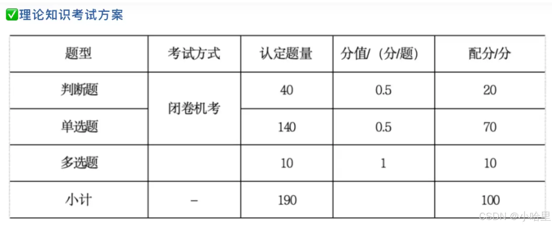
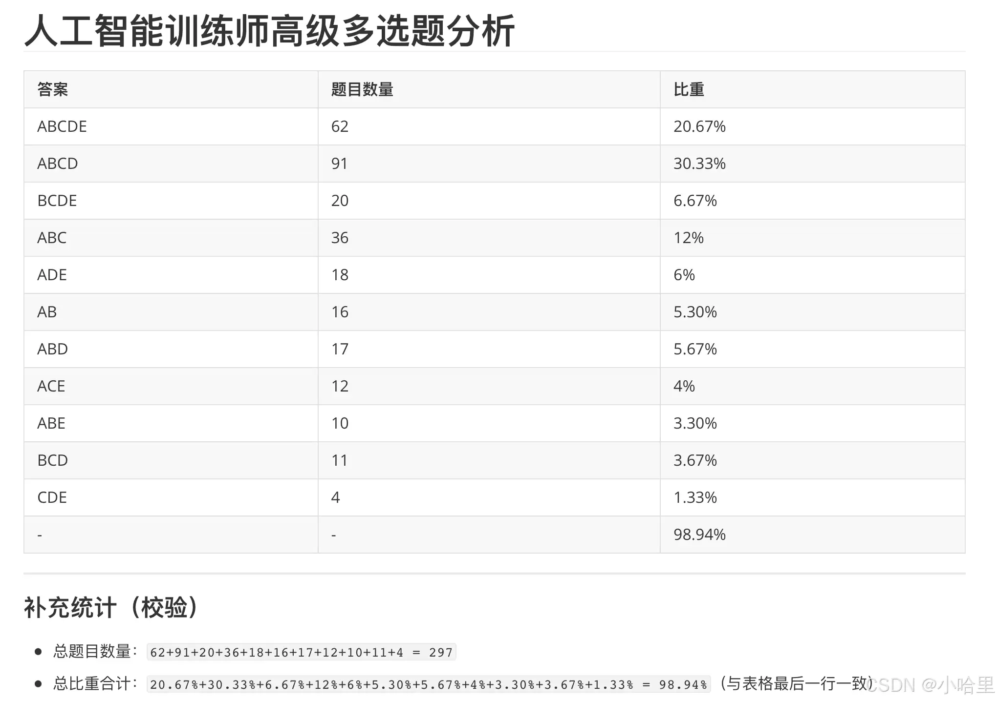

Copyright(C) 2020-2026 jiyx.com All Rights Reserved 联系方式:[email protected]